From Bézier to Bernstein
Posted November 2008.
Bézier curves are ubiquitous in computer graphics. ...
Bill Casselman
University of British Columbia, Vancouver, Canada
cass at math.ubc.ca
Introduction
Bézier curves are ubiquitous in computer graphics. They were introduced implicitly into theoretical mathematics long before computers, primarily by the French mathematician Charles Hermite and the Russian mathematician Sergei Bernstein. But it was only the work of Pierre Bézier, an employee of the automobile maker Renault, and of Paul de Casteljau, of Citroen, that made these curves familiar to graphics specialists. Recently, the polynomials defined by Bernstein have become again of interest to mathematicians.
Bézier curves
 |
|
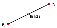
The simplest Bézier curve is the straight line from one point P0 to another P1, with the parametric equation
|
B(t) = P0 + t(P1 - P0) = (1-t) P0 + t P1
|
from which it follows immediately that
For t in between 0 and 1 the point B(t) is t of the way from one to the other. This is the same as the weighted average of the two points, with P0 given weight 1-t and P1 given weight t. When t=1/2, for example, B(t) is the point (1/2)(P0 + P1) halfway between P0 and P1.
|
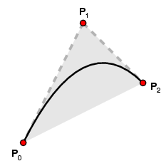
A quadratic Bézier curve is determined by three control points P0, P1, and P2. It has the parametric form
|
B(t) = (1-t)2 P0 + 2t(1-t) P1 + t2 P2
|
When t=0 all but terms but the first vanish, and when t=1 all but the last vanish. Therefore
The velocity vector at t is
|
B'(t) = -2(1-t)P0 + 2 (1-t)P1 - 2 t P1 + 2t P2 = 2 [ (1-t) (P1-P0) + t (P2-P1) ] .
|
When t=0 the velocity vector is 2(P1-P0) and when t=1 it is 2(P2-P1). Thus, the path starts at P0, ends at P2, and its tangents at P0 and P2 intersect at P1.
|
|
 |
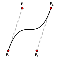
A cubic Bézier curve is determined by four control points P0, P1, P2, and P3. It has the parametric form
|
|
B(t) = (1-t)3P0 + 3 t(1-t)2P1 + 3t2(1-t) P2 + t3P3
|
|
|
 |
 |
Again, B(0) = P0 and B(1) = P3.
The velocity vector at t is
|
B'(t) = 3 [ (1-t)2(P1-P0) + 2t(1-t)(P2_P1) + t2(P3-P2) ].
|
When t=0 the velocity vector is 3(P1-P0) and when t=1 it is 3(P3-P2). Thus, the path starts at P0, ends at P3; when it leaves P0 it is heading towards P1, and when it arrives at P3 it is coming from the direction of P2. Otherwise, the relationship between the path and the control points is intuitively weak.
In all these cases, the coefficients of the points Pi in the parametric equation are terms which appear in the binomial expansion, respectively
|
(1-t), t
(1-t)2, 2t(1-t), t2
(1-t)3, 3t(1-t)2, 3t2(1-t), t3 .
|
|
For t between 0 and 1 these are non-negative, and by the binomial theorem the sum is [ t + (1-t) ]n = 1n = 1 for n=1, 2, 3. What this means is that each point B(t) is a weighted average of the control points, hence lies inside the convex hull of those points.
|
|
 |
 |
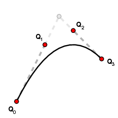
A Bézier curve of one degree can be reproduced by one of higher degree. For example, the quadratic Bézier curve with control points P0, P1, P2 is the same as the cubic Bézier curve with control points
|
Q0 = P0
Q1 = (1/3)P0 + (2/3)P1
Q2 = (2/3)P1 + (1/3)P2
Q3 = P2
|
|
|
|
 |
This can be checked by a simple algebraic calculation.
Calculus and Bézier curves
Suppose B(t) to be a cubic Bézier curve. We know that its coordinates are functions of t, and that position and velocity at endpoints are determined by the equations:
|
B(0) = P0
B'(0) = 3(P1-P0)
B'(1) = 3(P3-P2)
B(1) = P3 .
|
These conditions determine B(t) uniquely, because of a simple result first observed by the French mathematician Charles Hermite. The conditions above are really conditions on the coordinates of B(t), so the claim follows from this:
THEOREM.
Given numbers y0, v0, y1, v1, there exists a unique polynomial P(x) of degree 3 such that
|
P(0) = y0
P'(0) = v0
P(1) = y1
P'(1) = v1 .
|
We can guess a formula for P(t), from that of Bézier cubic curves:
|
P(t) = (1-t)3y0 + 3(1-t)2t [y0 + (1/3)v0] + 3(1-t)t2 [ y1 - (1/3)v1] + t3 y1 .
|
As for uniqueness, if we have two such polynomials, let D(x) = a + bx + cx2 + dx3 be their difference. Then
|
P(0) = a = 0
P'(0) = b = 0
P'(1) = b + 2c + 3d = 0
P(1) = a + b + c + d = 0 .
|
These tell us immediately that a=b=0, and these four equations immediately reduce to two:
which have only the solutions c=d=0. Q.E.D.
This is a special case of the main result of Hermite, according to which we may find a unique polynomial of degree n-1 satisfying a total of n conditions on values of the low order derivatives at possibly different points. This is called Hermite interpolation. This Theorem suggests a converse process. Suppose we are given a formula for a function f(x), as well as a formula for its derivative f'(x), and suppose we want to graph the function in a range a ≤ x ≤ b. We could just draw a bunch of very small line segments, but we can get a smoother curve by using Bézier cubic curves. Because if we are given a mediumly small range [c, d] it seems like a reasonable idea to approximate the function over that range by a cubic polynomial P(x) that satisfies these conditions:
|
P(c) = f(c)
P'(c) = f'(c)
P'(d) = f'(d)
P(d) = f(d) .
|
To see how Hermite's result applies, replace P varying over the range [c,d] by Q(t) where t varies over [0,1], and with
|
Q(t) = P((1-t)c + td), P(x) = Q((x-c)/(d-c)) .
|
To this Q we can apply Hermite's formula. A little algebra will then show that the graph between c and d will be approximated by the Bézier cubic with control points
|
(c, f(c))
(c + h/3, f(c) + (h/3)f'(c))
(d - h/3, f(d) - (h/3)f'(d))
(d, f(d))
|
where h=d-c.
There is one situation where this technique is definitely a good idea. Suppose that

where we do not have a formula for the indefinite integral of g(x). For example, we might have

Then we must approximate the integral numerically, say by Simpson's rule, so we have a recursive estimate
|
f(x+h) = f(x) + (h/6) ( g(x) + 4 g(x + h/2) + g(x+h) )
|
and, by the Fundamental Theorem of Calculus, the graph between x and x+h for small h is approximated by the Bézier curve with control points
|
(x, f(x))
(x + h/3, f(x) + (h/3)g(x))
(x + 2h/3, f(x+h) - (h/3)g(x+h))
(x + h, f(x+h))
|
where the last is computed according to Simpson's rule.
The same idea can be nicely used to plot the trajectories of systems of differential equations in the plane, using a numerical approximation to go from f(x) to f(x+h), such as one of the Runge-Kutta formulas.
Why Bézier curves?
There is something at first a bit odd about cubic Bézier curves, the fact that the curves don't actually go through the control points. So let's imagine an alternate way to draw curves that go nicely from one point P0 to another point P3, with a cubic parametrization P(t). The only technique that suggests itself naturally is choosing two points P1 and P2, and having the curve pass through them, not just near them as Bézier curves do. This means also choosing parameter values t1 and t2 with P(t1) = P1 and P(t2) = P2. The first choice that comes to mind is t1 = 1/3, t2=2/3. But it is well known (and explained clearly in the book by Henrici referred to later) that the curves chosen in this way look very odd. What turns out to be more reasonable is to choose t1 closer to 0, t2 closer to 1. But this means that we are very close to fixing values of the velocity at 0 and 1, which is essentially what Bézier curves do.
|

|
|
The deciding factor in choosing Bézier curves is a recursive property that makes them extremely efficient to compute. There is an algorithm attributed to de Casteljau that draws them very quickly. This depends on a certain recursive property. Suppose we are given a quadratic Bézier curve with control points Pi. Let's now divide it up into two halves, with P012 = B(1/2). Let P01 be the point midway between P0 and P1 , P12 be that midway between P1 and P2. In these circumstances: (1) the point P012 is the point midway between P01 and P12 ; (2) the half curve between P0 and the midpoint P012 is again a quadratic Bézier curve with control points P0 , P01 , and P012. Similarly for the second half.
|
|
Therefore, in order to draw the curve the computer can keep calculating midpoints - very easy to do on modern binary machines since it involves division by 2 - until it has broken the curve into a number of small segments that are essentially straight, and then it can draw all those as straight line segments. Something very similar happens for cubic Bézier curves, too - each half of a cubic Bézier curve is a Bézier curve with easily calculated control points, as the neighboring figure illustrates.
|
|

|
Bézier curves and fonts
One of the most common uses of Bézier curves is in the design of fonts. Cubic Bézier curves are used in Type 1 fonts, and quadratic Bézier curves are used in True Type fonts. Cubic Bézier curves are also used in the TEX fonts designed by Donald Knuth, and one of the clearest explanations is in his book MetaFont: the Program.
Bernstein polynomials
The formulas for the coordinates of Bézier curves
|
B1(t) = (1-t) x0 + t x1
B2(t) = (1-t)2 x0 + 2 (1-t)t x1 + t2 x2
B3(t) = (1-t)3 x0 + 3 (1-t)2t x1 + 3(1-t)t2 x2 + t3 x3
|
are special cases of a more general formula for polynomials of all degrees
|
Bn,x(t) = (1-t)n x0 + n (1-t)n-1t x1 + n(n-1)/2 (1-t)n-2t2 x2+ ... + Cn,k (1-t)n-ktk xk + ... + tn xn
|
where Cn,k is the binomial coefficient n!/k!(n-k)! Thus Bn,x (0)= x0, Bn,x(1) = xn. Here x is the array (xi).
These polynomials were first defined by the Russian mathematician Sergei Bernstein around 1910. The coefficients of a Bernstein polynomial of degree n are the coefficients in the binomial expansion of [(1-t) + t]n. They are all non-negative, and their sum is 1. The value of Bn(t) is therefore a weighted average of the numbers xi in the array x. The term Cn,k (1-t)n-ktk is also the probability of k successes in n trials in which the probability of a success is t. This is not an unimportant fact, as we shall see. They have a number of fundamental properties that we have seen already for Bézier curves:
|
The derivative of Bn,x(t) is B'n,x(t) = nBn-1,dx(t) where dx is the array of differences (xi+1-xi).
|
Thus both B'n,x(0) and B'n,x(1) have simple expressions. Otherwise, the exact relationship between the polynomial and its control values is rather obscure. One other useful feature is that
|
The graph of y = Bn,x(t) for t between 0 and 1 lies inside the convex hull of the points (k/n, xk).
|
A related fact, which is crucial in the application of Bernstein polynomials to optimization problems:
|
The maximum and minimum values of Bn,x(t) in [0,1] are bounded by the maximum and minimum values of its coefficients.
|
And here is the proper generalization of de Casteljau's algorithm:
|
The restrictions of Bn,x(t) to each half-range [0,1/2] and [1/2,1] are also Bernstein polynomials, in the sense that each of Bn,x (2t) and Bn,x (1-2t) can be expressed as Bn,y (t) for some array y that is simple to calculate.
|
These polynomials were invented by Sergei Bernstein in order to prove a fundamental result in approximation theory, as we shall see in the next section. They are impractical in this role, but in recent years they have proven important in optimization theory. See, for example, the thesis of Roland Zumkeller (linked to in the References). This is gratifying - almost anyone who has seen Bernstein's proof of Weierstrass' theorem must have felt that these polynomials were destined to play other roles, as well.
Bernstein's proof of Weierstrass' approximation theorem
In about 1885 Karl Weierstrass, at the age of 70, published a proof of one of the theorems for which he is most famous: Any continuous function on the interval [0,1] may be uniformly approximated, arbitrarily closely, by polynomials. The definition of continuous functions is relatively simple, and this definition is in close accord with intuition, so it was apparently surprising to learn, as mathematicians of the nineteenth century acquired more and more knowledge about them, that continuous functions could exhibit rather strange behavior. Weierstrass' theorem was perhaps considered refreshing evidence that they were not so wildly behaved after all.
Many outstanding mathematicians soon came up with proofs rather different from Weierstrass' original one. One of the most satisfying was that found by Sergei Bernstein, and it was apparently for this purpose that he came up with the polynomials now named after him. Unlike other versions, his provides a very explicit converging sequence of polynomials.
Suppose f is a continuous function on [0,1]. For each n let fn be the array of n+1 values f(k/n) for k = 0, ..., n. Explicitly, we have
|
Bn,f (t) = Bn, fn (t) = f(0) (1-t)n + f(1/n) n (1-t)n-1 t + ... + f(k/n) Cn,k (1-x)n-ktk + ... + f(1) tn
|
THEOREM. Suppose f(x) to be a continuous function on [0,1]. The polynomials Bn,f (x) converge uniformly on [0,1] to f(x) as n goes to infinity.
|
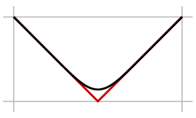
Here for example, is Bernstein's approximation to f(x) = |x-1/2| for n=32:
|
|
 |
and here is a table of the Bernstein approximations of |t-1/2| at t=1/2 for various values of n:
|
n
|
Bn,f (1/2)
|
|
4
|
0.1367
|
|
8
|
0.0982
|
|
16
|
0.0700
|
|
32
|
0.0497
|
|
64
|
0.0352
|
|
128
|
0.0249
|
As you can guess, the convergence here is of order about 1/n1/2 around t=1/2, and better at other points. We can see that although one virtue of Bernstein polynomials is that they can approximate arbitrary continuous functions, on functions that one sees in practice they converge at an impractically slow rate.
Bernstein's proof of convergence is very elegant. It is a variation on a simple argument used in a slightly different context, that of local averaging. Suppose f to be a continuous function on [0,1]. Define for each n a function
|
fn(x) = (1/2)( f(x - 1/2n) + f(x + 1/2n) ) .
|
In other words, the value of fn at x is the average of its values at x-1/2n and x+1/2n, an interval of width 1/n. Or, to give slightly more complicated examples:
|
fn(x) = (1/4)( f(x - 1/n) + 2 f(x) + f(x + 1/n) )
|
or
|
fn(x) = (1/8) ( f(x - 3/2n) + 3 f(x - 1/2n) + 3 f(x + 1/2n) + f(x + 3/2n) ) .
|
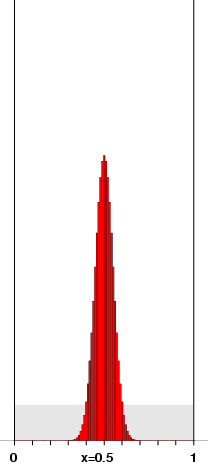
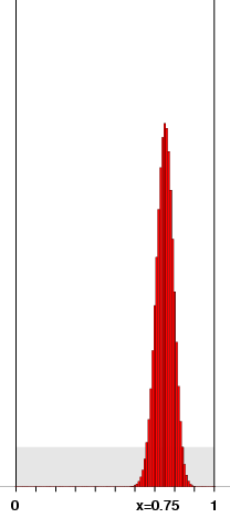
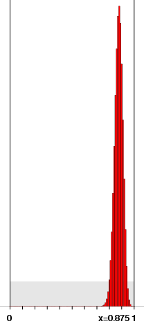
These are now different weighted averages of f near x. Bernstein's definition of fn(x) is also a weighted average of values of f around x, but the weighting depends on x. The value of the polynomial Bn,f at x is also a weighted average of f around x, although that is not at all apparent at first sight. It is a sum of values of f at certain point k/n, and what happens is that only the terms for k/n near x make a sizable contribution. Here are some graphs of the weighting for various values of x, with n=100:


Why is this? The weighting function is the distribution of k successes in n trials with a probability of success equal to x. The average number of successes - the mean value of this probability distribution - is x, and the real basis of Bernstein's reasoning is that the standard deviation of this distribution - the quantitative measure of its spread - is
As n grows, this shrinks. What this means is that the probability distribution clusters more narrowly around the mean value x, and more or less uniformly for all x. The proof uses this observation. Since the sum of the binomial coefficients is 1, we have
|
| f(x) - Bn, fn(x) | ≤ Σk | f(x) - f(k/n) | Cn,k (1-x)n-k xk
|
We can divide the sum over the point k/n into those which are near x and those far away, since we expect the sum over the near ones will be the major contribution. Say we choose some small number δ and sum over k/n with |x-k/n| ≤ δ and those with |x-k/n| > δ.
The first is
|
Σ|x-k/n| ≤ δ | f(x) - f(k/n) | Cn,k (1-x)n-k xk .
|
If we choose δ small enough so | f(x) - f(k/n) | < ε/2 whenever |x - k/n| ≤ δ, this will be less than ε/2.
Now let let M be the maximum spread of f on [0,1]. The second sum is
|
Σ|x-k/n| ≤ δ | f(x) - f(k/n) | Cn,k (1-x)n-k xk
|
which is at most M times the sum
|
Σ|x-k/n| > δ Cn,k (1-x)n-k xk .
|
We must now choose n so that this sum is at most ε/2M. Being able to do so is plausible, since as n increases the range over which Cn,k (1-x)n-k xk is sizable becomes narrower. There are many ways to make this idea rigorous - the simplest is to use Chebyshev's inequality. This says that if pi is a discrete probability distribution with mean m and standard deviation σ then the probability of |t - m| ≥ s σ is at most 1/s2. This is a very elementary fact, and we'll come back to justify it in a moment. Given it, we see that if n > 2M x(1-x) / ε δ2 then the sum above is less than ε/2.
Proof of Chebyshev's inequality. Since |t - m|/ sσ > 1 if and only if |t - m|2/s2 σ2 > 1, the sum is that of all pi over all ti with |ti - m|2/s2 σ2 ≥ 1. But this is at most the sum of |ti-m|2/s2σ2 over the same region, which is in turn is at most the sum over all i of the same terms, which is (by definition of standard deviation)
|
Σi pi ( |ti - m|2/s2 σ2 ) = ( 1/s2 σ2 ) Σi pi |xi - m|2 = 1/s2
|
References
To find out more ...
... about Bézier curves
The first two books contain articles by Pierre Bézier on the history of his work with the curves named after him.
- R. E. Barnhill and R. F. Riesenfeld (editors), Computer Aided Geometric Design, Academic Press, 1974.
This book contains papers presented at a conference at the University of Utah that initiated much of modern computer graphics.
- G. Farin, Curves and surfaces for computer aided design, Academic Press, 1988.
Various works by Donald Knuth explain clearly the role of Bézier curves in font design.
- D. E. Knuth, MetaFont: the Program, Addison-Wesley, 1986.
The source code for this book is in the WEB file mf.web available in CTAN distributions, and in particular at http://www.ctan.org/tex-archive/systems/knuth/dist/mf/. This can be turned to a TEX file by applying the program weave. Pages 123 - 131 explain extremely clearly the author's implementation of Bézier curves in his program MetaFont. For the admittedly rare programmer who wishes to build his own implementation (at the level of pixels), or for anyone who wants to see what attention to detail in first class work really amounts to, this is the best resource available.
- MetaFont (Wikipedia)
- MetaFont: the Book (TEX source)
Be sure also to download the macros necessary to TEX it.
The next two items are about interpolation of various kinds.
- Charles Hermite, "Sur la formule d'interpolation de Lagrange", Journal für die reine und angewandte mathematik, volume 84, 1877.
This is available from the Göttingen Digital Archive.
- Peter Henrici, Essentials of numerical analysis, Wiley, 1982
Discusses interpolation and the related topic of splines very clearly.
... about Bernstein polynomials
Wikipedia has several useful entries involving Bernstein polynomials and interpolation.
There is a major site at Technion University concerned with approximation theory:
Bernstein polynomials are not practical for polynomial approximation, but in recent years it has become apparent that they are practical for optimization. The next item is one of the more interesting places where this is discussed.
- Roland Zumkeller's web pages
Zumkeller's thesis Global optimization in type theory is available in the publications list. It explains the role of Bernstein polynomials in a project to provide provable estimates of the minimal value of a polynomial on certain domains. This is part of a larger project to produce a formal proof of of Kepler's conjecture along the lines of Thomas Hales' proof. His exposition of the theory of Bernstein polynomials is novel.
Bill Casselman
University of British Columbia, Vancouver, Canada
cass at math.ubc.ca
Those who can access JSTOR can find some of the papers mentioned above there. For those with access, the American Mathematical Society's MathSciNet can be used to get additional bibliographic information and reviews of some these materials. Some of the items above can be accessed via the ACM Portal , which also provides bibliographic services.


