That Knotty DNA

David Austin
Grand Valley State University
david at merganser.math.gvsu.edu

Mail to a friend

Print this article

Introduction

Gardening presents a mathematical challenge for me: As I drag the garden hose around my lawn, the hose invariably gets tangled up with itself in ways that can seem endlessly complicated. Untangling the hose usually requires time and patience; the job would be a lot easier if I could somehow pass the hose through itself to untangle it.

Still, my garden hose is nothing compared to the complexity of DNA in the nucleus of a cell. For example, imagine the nucleus of a cell scaled to the size of a basketball. The DNA contained inside would form a 200 kilometer long double-stranded filament tightly knotted inside. Now think about what happens when a cell divides: A second copy of the DNA is produced, which is necessarily tangled up with the first, and this copy must somehow be pulled apart from the original.

Enzymes, known as topoisomerases, assist by breaking and rejoining strands of DNA; in essence, topoisomerases allow the molecules to pass through one another, just as I wish for my garden hose. These enzymatic actions are of great interest to molecular biologists, who have spent considerable effort exploring them experimentally. To detect changes effected by the enzymes, however, we need some way to compare the knottedness of two molecules. This is where mathematics comes in.

The study of knots began in earnest in the 1860's when William Thompson (Lord Kelvin) proposed his vortex model of the atom. Simply said, this theory postulated that atoms were formed by knots in the ether and that different chemical elements were formed by different knots. Though Kelvin's theory eventually proved to be of little physical use, it was seriously considered for long enough to lead mathematicians to begin a detailed study of knots.

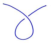
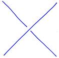
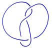
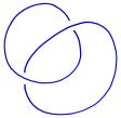
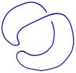
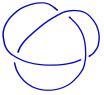
Of particular interest to mathematicians is the problem of determining whether two knots, like the ones shown below, are the same or different. That is, can we reconfigure one of the knots, without cutting, so that it looks like the other?

Knots are phenomenally complicated: if we just look at knots that appear to cross 16 times or less, we find that there are 1,388,705 different knots. Since Kelvin's time, mathematicians have developed increasingly powerful tools for making sense of this complexity. In this article, we'll look at one tool, the Jones polynomial, which has been used by molecular biologists in their investigations of DNA.

Naming knots

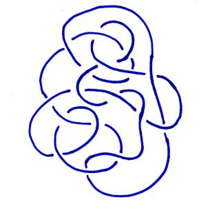
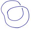
One problem with knots is that there are many ways to look at them; what appears complicated at first sight could simply be due to our misfortune at having looked in the wrong way. For instance, the two knots below are really the same though one appears, at least at first glance, to be a more complicated knot.

To distinguish knots from one another, mathematicians have developed ways to assign names to knots, just the way that people have names assigned to them. Of course, people with different names are different; in the same way, knots with different names are different as well. In the 1980's, Vaughn Jones found a way to name knots by associating a polynomial, now called the Jones polynomial, to every knot. This is a particularly powerful way to name knots for it distinguishes many knots from one another. The Jones polynomials are shown for the knots below. As you can see, the polynomials are different and so the knots themselves must be different.

	V(t) =t+t3-t4,
	V(t) =t2-t+1-t-1+t-2.

Rather surprisingly, Jones found his polynomial through his work in operator algebras, an area of mathematics seemingly far-flung from knot theory. In this article, we'll follow a path to the Jones polynomial found by Louis Kauffman.

Link diagrams

Let us restate a fundamental difficulty in dealing with knots: different pictures of the same knot may look wildly different. However, a theorem proved by Kurt Reidemeister in the 1930's gives us a way to understand how different pictures of the same knot may vary from one another.

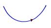
In what is coming, we will need to work with links, which are merely collections of knots. The following three simple changes, called Reidemeister moves, may be made to the picture of a link without changing the link itself.

	Move I
	Move II
	Move III

If we are given two pictures of the same link, Reidemeister's theorem guarantees that there is a sequence of these three moves that lead from one picture to the other. The example below illustrates:

	Move II		Move I
	Move III		Move III

The Kauffman and Jones polynomials

As we'll now see, Kauffman began by associating a polynomial, called the bracket polynomial, in variables x, y, and z to the picture of a link. For instance,

= (x2+y2)z + 2xy

The bracket polynomial is defined by three simple rules.

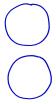
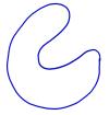
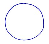
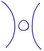
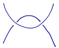
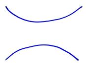
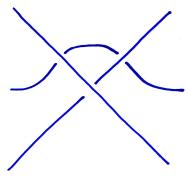
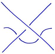
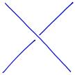
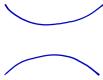
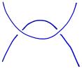
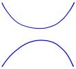
1. First, we will assign a simple polynomial to the unknot: = 1 2. Our strategy will be to compute the polynomial by eliminating crossings: = x + y 3. We will also eliminate circles from the link diagrams. If D is a diagram and one circle is added to the diagram, then + D = z D

---

Let's see how this works in the following example:

	= x		+ y
	= x2		+ xy
	+ yx		+ y2
	= (x2+y2)z		+ 2xy
	= (x2+y2)z + 2xy

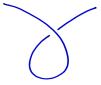
Remember that we would like to have a polynomial that depends only on the underlying link, rather than the diagram we are using to represent it. This would be the case if the polynomial is unchanged when we perform any of the three Reidemeister moves. Considering the first Reidemeister move, we would therefore like to have

=

Let's see where this leads us:

	= x		+ y
	= x2		+ xy
	+ yx		+ y2
	= xy		+ (x2+y2+xyz)

Since we would like

=

we must have

xy = 1
x² + y² + xyz = 0.

In other words,

y = x^-1
z = -(x² + x^-2)

Let's revise our three rules now:

= 1 = x + x-1 + D = -(x2 + x-2) D

With these new rules, it turns out (remarkably) that the bracket polynomial is unchanged by the second Reidemeister move:

=

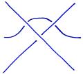
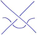
Now we need to check the third Reidemeister move:

	= x		+ x-1
	= -x(x2+x-2)		+ x-1
	= -x3

This looks like a problem. We would like for the bracket polynomial to be unchanged under all three Reidemeister moves. Moves I and II leave it unchanged, but straightening out the kink in move III introduces a factor of -x³.

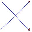
Fortunately, there is a way to fix this problem. To do so, we will first orient the link diagram by putting arrows on it:

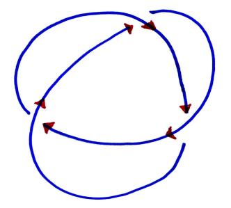
and define the incidence number of a crossing to be:

+1 if the crossing is like
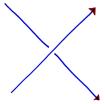-1 if the crossing is like

The writhe of the diagram is now the sum of all the incidence numbers. You may wish to check that the writhe of a knot diagram does not depend on how we oriented the knot. Notice that Reidemeister move III changes the writhe:

writhe

+ 1 = writhe

Therefore, if we have an oriented link diagram L and define the polynomial P_L(x) to be

PL(x) = (-x3)writhe(L)

L

then this polynomial depends only on the oriented link and not on the diagram used to represent it. In other words, everyone who draws a picture of this link will still compute the same polynomial regardless of how his or her picture looks. Also, if L is a knot, then the polynomial does not depend on the orientation since the writhe is independent of the orientation.

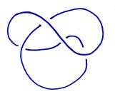
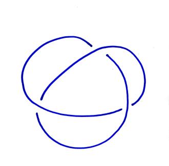
A good exercise is to compute the polynomial for the trefoil knot:

PT(x) =x-4+x-12-x-16,

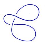
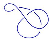
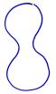
or the figure 8 knot:

P8(x) =x8-x4+1-x-4+x-8.

This polynomial, known as the Kauffman polynomial, is related to the Jones polynomial, which predates it. The Jones polynomial is given by

Chirality

Molecules often occur in pairs, each of which is the mirror image of the other, and biologists would like to distinguish between them. The Jones polynomial is also helpful here.

Imagine looking at a link in a mirror that is directly behind the link. We would see the same link diagram, but the over- and under-crossings would simply be interchanged. For instance, here is a trefoil knot and its mirror image:

Let's first consider the effect of interchanging an over- and under-crossing on the bracket polynomial:

	= x		+ x-1
	= x-1		+ x

Also, interchanging over- and under-crossings will change the sign of all the incidence numbers

so the writhe changes sign.

Putting these two observations together means that if is the mirror image of the oriented link L, then

and hence

Consider now the trefoil and its mirror image:

V(t) =t+t3-t4	V(t) =t-1+t-3-t4

Since the two polynomials are different, this shows that the trefoil and its mirror image are two different knots. That is, there is no way to deform the trefoil into its mirror image without cutting it apart and tying it back together.

You may wonder about the figure 8 knot, since its polynomial is

This tells us that the Jones polynomial cannot distinguish between the figure 8 knot and its mirror image. It turns out that the figure 8 knot is equivalent to its mirror image, a fact that you may wish to verify by finding a sequence of Reidemeister moves that takes the picture of the figure 8 knot into its mirror image.

Summary

After Kelvin's vortex theory was abandoned as an explanation for atomic structure, mathematicians studied knots for over a century motivated mainly by curiosity. In some sense, Jones's work represents the culmination of this work for it seems to bring together several areas of mathematics. As mentioned, Jones's original motivation came from operator algebras. In addition, the Jones polynomial forms rather deep connections between knot theory and statistical mechanics and quantum field theory.

Also unexpected is its usefulness in studying the chemical processes of life. Nicholas Cozzarelli, a molecular biologist at the University of California-Berkeley until his death last year, said: "Before Jones, the math was incredibly arcane. The way the knots were classified had nothing to do with biology, but now you can calculate the things important to you".

This phenomenon is not uncommon. New mathematics is often discovered out of simple curiosity yet is indispensable for describing the world around us.

References

Knot theory references accessible to undergraduates.

Standard references on knot theory

More specific references to the Kauffman and Jones polynomials

Connections between biology, chemistry and knot theory

David Austin
Grand Valley State University
david at merganser.math.gvsu.edu

NOTE: Those who can access JSTOR can find some of the papers mentioned above there. For those with access, the American Mathematical Society's MathSciNet can be used to get additional bibliographic information and reviews of some these materials. Some of the items above can be accessed via the ACM Portal, which also provides bibliographic services.