Abstract

Bézier control points method to solve constrained quadratic optimal control of time varying linear systems

F. Ghomanjani; M.H. Farahi; M. Gachpazan

Department of Applied Mathematics, Faculty of Mathematical Sciences, Ferdowsi University of Mashhad, Mashhad, Iran. E-mail: gachpazan@ferdowsi.um.ac.ir

ABSTRACT

A computational method based on Bézier control points is presented to solve optimal control problems governed by time varying linear dynamical systems subject to terminal state equality constraints and state inequality constraints. The method approximates each of the system state variables and each of the control variables by a Bézier curve of unknown control points. The new approximated problems converted to a quadratic programming problem which can be solved more easily than the original problem. Some examples are given to verify the efficiency and reliability of the proposed method.

Mathematical subject classification: 49N10.

Key words: Bézier control points, constrained optimal control, linear time varying dynamical systems.

1 Introduction

In the numerical solution of differential equations, polynomial or piecewisepolynomial functions are often used to represent the approximate solution [1] . Legendre and Chebyshev polynomials are used for solving optimal control problems (see [2] , [3] , [4] and [5] ). Razzaghi and Yousefi [6] defined functions which they called Legendre wavelets for solving constrained optimal control problem. In particular, B-splines and Bezier curves have become popular tools for solving dynamical systems [7] . For both Bezier and B-spline representations, the curve or surface shape is outlined by a "control polygon" that is formed by connecting the control points. Since the control point structure captures important geometric features of the Bezier or B-spline shape, it is tempting to perform computations just based on the control points. This paper intends to investigate the use of the control points of Bezier representations for solving optimal control problems with inequality constrained. Since the use of B-splines is to cause the continuity of control curves, we propose to represent the approximate solution in Bezier curves for time varying optimal control problem with inequality constraints. The choice of the Bezier form rather than the B-spline form is due to the fact that the Bezier form is easier to symbolically carry out the operations of multiplication, composition and degree elevation than the B-spline form. We choose the sum of squares of the Bezier control points of the residual to be the measure quantity. Minimizing this quantity gives the approximate solution. Obviously, if the quantity is zero, then the residual function is also zero, which implies the solution is the exact solution. We call this approach the control-point-based method.

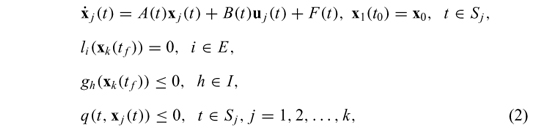
Consider the following time varying optimal control problem with pathwise state inequality constraints,

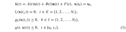
where

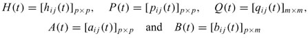
are matrices functions and K(t) = (k₁(t) ... k_p(t)), R(t) = (r₁(t) ... r_m(t)), F(t) = (f₁(t) ... f_p(t))^T are vectors functions, where the entries of mentioned matrices and polynomials in [t₀, t_f] . One may note when the entries of mentioned matrices are not polynomials in [t₀, t_f] , Taylor series is used for approximation. x(t) = (x₁(t) x₂(t) ... x_p(t))^T∈ R^p is p ×1 trajectory state vector, u(t) ∈ = {(u₁(t) u₂(t) ... u_m(t))^T : < u_i < , 1 < i < m} ⊆ R^m is m × 1 control vector. The fixed finite terminal time t_f is given, and x₀ is the vector of initial conditions. In addition, l_i : R^p → R for i ∈ E, g_h : R^p → R for h ∈ I, q : [t₀, t_f] × R^p → R, and , , 1 < i < m are given bounded functions.

The constrained optimal control of a linear system with a quadratic performance index has been of considerable concern and is well covered in many papers (see [6] and [8] ). One of the methods to solve constrained optimal control problem (1), based on parameterizing the state/control variables, which convert the problem to a finite dimensional optimization problem, i.e. a mathematical programming problem (see [9] , [10] , [11] -[16] ).

Analytical techniques developed in [5] are of benefit also in studying the convergence properties of related algorithms for solving optimal control problems, involving Chebyshev type functional constraints where, owing to the use of a variable step-size in integration or high order integration procedures, it is either not possible or inconvenient to base the analysis on an a priori discretization of the dynamic. The method used slack variables to convert the inequality constraints into equality constraints. This approach has an obvious disadvantage when applied to constrained optimal control of time varying linear problems because it converts the linear constraints into a nonlinearone (see [17] ).

In this paper, we show a novel strategy by using the Bézier curves to find the approximate solution for (1). In this method, we divided the time interval, into k subintervals and approximate the trajectory and control functions in each subinterval by Bézier curves. We have chosen the Bézier curves as piecewise polynomials of degree n, and determine Bézier curves on any subinterval by n + 1 control points. By involving a least square optimization problem, one can find the control points, where the Bézier curves that approximate the action of control and trajectory, can be found as well (see [7] and [18] ).

To show the effectiveness of this method the computational results of threeexamples are presented and compared with the results obtained in [5] and [17] .

2 Least square method

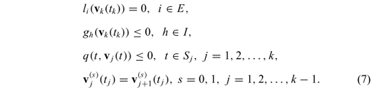
Let k be a chosen positive integer and {t₀ < t₁ < ... < t_k = t_f} be an equidistance partition of [t₀, t_f] with length τ and S_j = [t_{j - 1}, t_j] for j = 1, 2,..., k. We define the following suboptimal control problems

where C_jk = (t_f)H(t_f)x_k(t_f), and δ_jk is the Kronecker delta whichhas the value of unity when j = k and otherwise is zero.

are respectively vectors of x(t) and u(t) when are considered in S_j = [t_{j - 1}, t_j] .

Our strategy is using Bezier curves to approximate the solutions x_j(t) and u_j(t) by v_j(t) and w_j(t) respectively, where v_j(t) and w_j(t) are given below. Individual Bezier curves that are defined over the subintervals are joined together to form the Bezier spline curves. For j = 1, 2,..., k, define the Bezier polynomials of degree n that approximate the actions of x_j(t) and u_j(t) over the interval S_j = [t_{j - 1}, t_j] as follows:

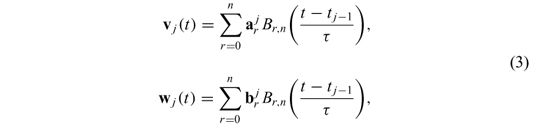
where

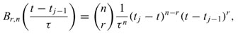
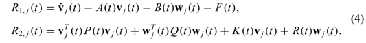
is the Bernstein polynomial of degree n over the interval [t_{j - 1}, t_j] , and are respectively p and m ordered vectors from the control points. By substituting (3) in (2), one may define residual R_{1, j}(t) and R_{2, j}(t) for t ∈ [t_{j - 1}, t_j] as:

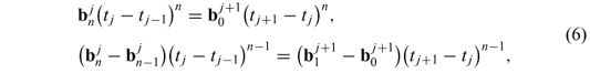
Beside the boundary conditions on v(t), in nodes, there are also continuity constraints imposed on each successive pair of Bezier curves. Since the differential equation is of the first order, the continuity of x (or v) and its first derivativegives

where (t_j) is the s-th derivative of v_j(t) with respect to t at t = t_j.

Thus the vector of control points (for r = 0,1, n - 1 and n) must satisfy

One may recall that is an p ordered vector. This approach is called the subdivision scheme (or τ-refinement in the finite element literature), in the Section 3, we prove the convergence in the approximation with Bezier curves when n tends to infinity.

Note 1: If we consider the C¹ continuity of w, the following constraints will be added to constraints (5),

where the so-called is an m ordered vector.

Now, we define residual function in S_j as follows

where ||.|| is the Euclidean norm (Recall that R_{1, j}(t) is a p vector where t ∈ S_j) and M is a sufficiently large penalty parameter. Our aim is to solve the following problem over ,

The mathematical programming problem (7) can be solved by many subroutines, we used Maple 12 to solve this optimization problem.

Note 2: If in time varying optimal control problem (1), x(t_f) be unknown, then we set C_kk = 0.

Note 3: To find good polynomial approximation, one needs to increase the degree of polynomial, in this article, we used sectional approximation, to find accurate results by low degree polynomials.

3 Convergence analysis

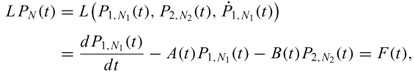
In this section, we analyze the convergence of the control-point-based method when applied to the following time varying optimal control problem:

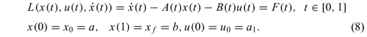
where the state x(t) ∈ R, u(t) ∈ R, a, b ∈ R, H(t), P(t), Q(t), K(t), R(t), A(t), B(t) and F(t) are polynomials in [0,1] .

Without loss of generality, we consider the interval [0,1] instead of [t₀, t_f] , since one can change the variable t with the new variable z by t = (t_f - t₀) z + t₀ where z ∈ [0,1] .

Lemma 3.1. For a polynomial in Bezier form

we have

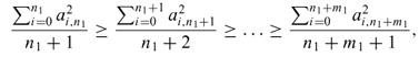
where a_{i,n1 + m1} is the Bezier coefficients of x(t) after it is degree-elevated to degree n₁ + m₁.

Proof. See [1].

The convergence of the approximate solution could be done in two ways

In the following we prove the convergence in each case.

3.1 Degree raising case

Theorem 3.2. If time varying optimal control problem (8) has a unique, C¹ continuous trajectory solution , C⁰ continuous control solution , then the approximate solution obtained by the control-point-based method converges to the exact solution as the degree of the approximate solution tends to infinity.

Proof. Given an arbitrary small positive number ε > 0, by the Weierstrass Theorem (see [19] ) one can easily find polynomials Q1,N₁(t) of degree N₁ and Q2,N₂(t) of degree N₂ such that

where ||.||_∞ stands for the L_∞-norm over [0, 1] . Especially, we have

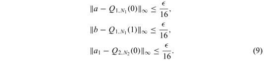
In general, Q1,N₁(t) and Q2,N₂(t) do not satisfy the boundary conditions. After a small perturbation with linear and constant polynomials αt + β and γ, respectively for Q1,N₁(t) and Q2,N₂(t), we can obtain polynomials P1,N₁(t) = Q1,N₁(t) + (αt + β) and P2,N₂(t) = Q2,N₂(t) + γsuch that P1,N₁(t) satisfy the boundary conditions P1,N₁(0) = a, P1,N₁(1) = b, and P2,N₂(0) = a₁. Thus Q1,N₁(0) + β = a, and Q1,N₁(1) + α + β = b. By using , one have

Since

so

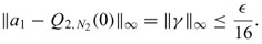
By the time, a₁ = P2,N₂(0) = Q2,N₂(0) + γ, so

Now, we have

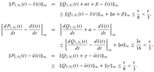
Now, let define

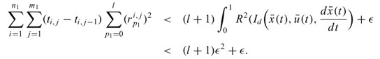
for every t ∈ [0, 1] . Thus for N > max{N₁, N₂}, one may find an upper bound for the following residual:

where C₁ = 1 + ||A(t)||_∞ + ||B(t)||_∞ is a constant.

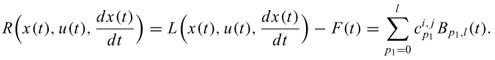
Since the residual R(P_N) : = LP_N(t) - F(t) is a polynomial, we can represent it by a Bezier form. Thus we have

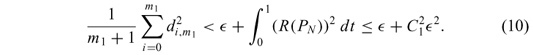
Then from Lemma 1 in [1] , there exists an integer M(> N) such that when m₁ > M, we have

which gives

Suppose x(t) and u(t) are approximated solution of obtained by the control-point-based method of degree m₂ (m₂> m₁> M). Let

Define the following norm for difference approximated solution (x(t), u(t)) and exact solution ((t), (t)):

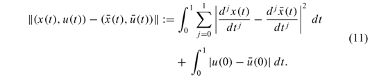
It is easy to show that:

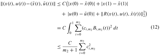
Last inequality in (12) is obtained from Lemma 1 in [1] in which C is a constant positive number. Now from Lemma 1 in [1] , one can easily show that:

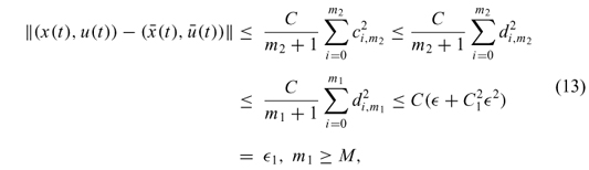
where last inequality in (13) is coming from (10).

Thus, from (13) we have:

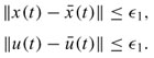
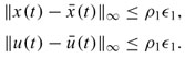
Since the infinite norm and the norm defined in (11) are equivalent, there is a ρ₁ > 0 where

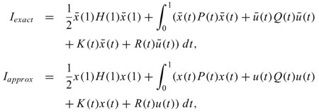
Now, we show that the approximated cost function tends to exact cost function as the degree of Bezier approximation increases. Define

for t ∈ [0, 1] . Now, there are four positive integers M_i > 0, i = 1,..., 6, such that

Since

we have

so

now, we have

This completes the proof.

3.2 Subdivision case

Theorem 3.3 Let (x, u) be the approximate solution of the linear optimal control problem obtained by the subdivision scheme of the control-point-based method. If has a unique solution (, ) where (, ) is smooth enough so that the cubic spline T(, ) interpolating to (, ) converges to (, ) in the order O(τ^q), (q > 2), where τ is the maximal width of all subintervals, then (x, u) converges to (, ) as τ → 0.

Proof. We first impose a uniform partition Π_d = ∪_i[t_i, t_{i + 1}] on the interval [0, 1] as t_i = id where d =

Let be the cubic spline over Π_d interpolating to (, ). Then for an arbitrary small positive number ε > 0, there exists a δ₁ > 0 such that

provided that d < δ₁. Let

be the residual. For each subinterval [t_i, t_{i + 1}] , is a polynomial. On each interval [t_i, t_{i + 1}] , we impose another uniform partition Π_i, τ = ∪_j [t_{i, j}, t_{i , j + 1}] as t_i,j = id + jτ where τ = , j = 0,..., m₁. Express in [t_{i, j - 1}, t_{i, j} ] as

By Lemma 3 in [1] , there exists a δ₂ > 0 (δ₂< δ₁) such that when τ < δ₂, we have

Thus

or

Now combining the partitions Π_d and all Π_i,τ gives a denser partition with the length τ for each subinterval. Suppose (x(t), u(t)) is the approximate solution by the control-point-based method with respect to this partition, and denote the residual over [t_{i,j - 1}, t_{i, j}] by

Then there is a constant C such that

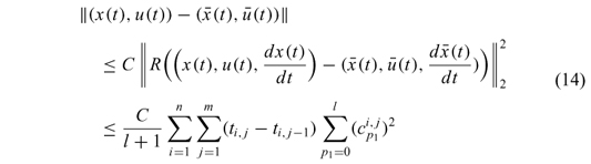
last inequality in (14) is obtained from Lemma 1 in [1] . One can easily show that:

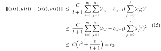
Thus, from (15) we have:

Since the infinite norm and the norm defined in (11) are equivalent, there is a ρ₂ > 0 where

Now, we show that the approximated cost function tends to exact cost function as the degree of approximation increases. Define

for t ∈ [t_{i,j - 1}, t_i,j] . Now, there are four positive integers M_i > 0, i = 1,..., 6, such that ||P(t)||_∞ < M₁, ||Q(t)||_∞ < M₂, ||K(t)||_∞ < M₃, ||R(t)||_∞ < M₄, ||(t)||_∞ < M₅, and ||(t)||_∞ < M₆. Since

we have

so

now, we have

Now, from Lemma 3 in [1] , we conclude that the approximated solution converges to the exact solution in order o(τ^q), (q > 2).

This completes the proof.

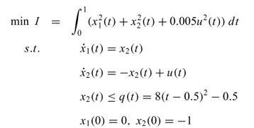
4 Numerical examples

Example 4.1. Consider the following constrained optimal control problem (see [5] ):

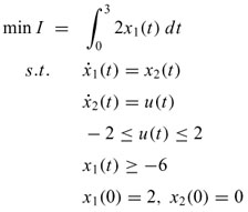
Let k = 6 and, n = 3, if one consider the C¹ continuity of u(t), one can find the following solution from (7)

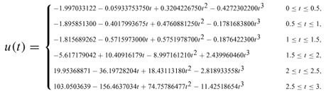
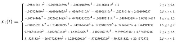
Then by involving the above control function u(.), in the indicated differential equation, one can find the trajectories x₁(.) and x₂(.) as follows:

and,

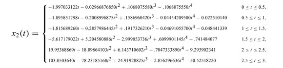
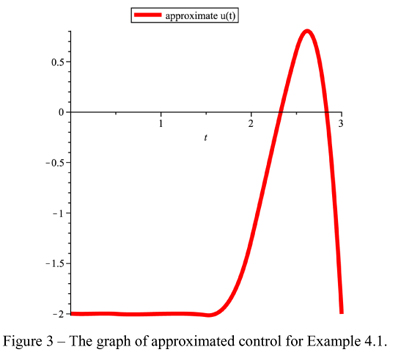
The graphs of approximated trajectories x₁(t) and x₂(t) are shown respectively in Figure 1 and Figure 2, and the graph of approximated control is shown Figure 3. The approximated and exact objective function are respectively I = -5.389857789, I^* = -5.528595476 (see [5] ).

In this example, we used Bezier polynomials of degree 10 to approximate the trajectories x₁(.) and x₂(.) through the time interval J = [0,3] , and without using subintervals. The objective function is found I = -5.360252730 and the trajectories x₁(t), and x₂(t) for t ∈ J are shown in Figures 4, 5. For reduction in complicated manipulations, the authors recommend to use low degree Bezier approximation polynomials and use subintervals approach.

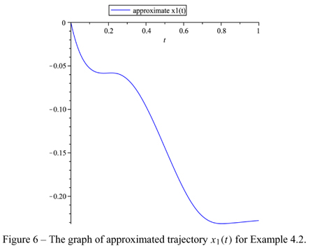
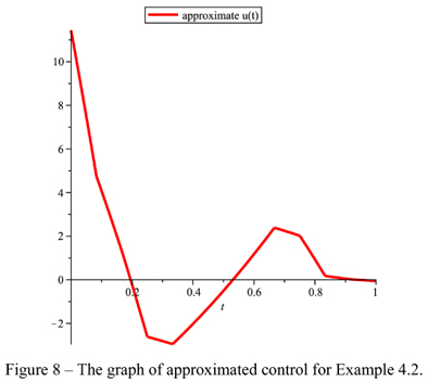
Example 4.2. Consider the following optimal control problem ([17] ):

Let k = 12, t₀ = 0, t_f = 1, t_j = t₀+ (j = 1,..., 12), and n = 3. From , one can find the following solution

The graphs of approximated trajectories x₁(t) and x₂(t) are shown respectively in Figure 6 and Figure 7, and the graph of approximated control is shown Figure 8. The approximated and exact objective function respectively are I = 0.1728904530, I^* = 0.17078488 (see [17] ). The computation takes 5 seconds of CPU time when it is performed using Maple 12 on an AMD Athelon X4 PC with 2 GB of RAM. The QPSolve command solves (7), which involves computing the minimum of a quadratic objective function possibly subject to linear constraints. The QPSolve command uses an iterative active- set method implemented in a built-in library provided by the numerical algorithms group.

5 Conclusions

In this paper, a Bézier control points method for solving optimal control problems governed by time varying linear dynamical systems with terminal state constraints and inequality constraints on the states and control has been suggested. The method replaces the constrained optimal control problem by a quadraticprogramming one, and the control point structure provides a bound on the residual function. The new mathematical programming problem is intuitive and easy to solve.

Numerical examples show that the proposed method is reliable and efficient. The control polygon gives an intermediate approximation to the appearance of the solution.

Acknowledgment. The authors like to express their sincere gratitude to referees for their very contractive advises.

Received: 01/VIII/11.

Accepted: 13/X/12.

#CAM-396/11.

Publication Dates

History