Squaring the Circle and Cubing the Sphere: Circular and Spherical Copulas

Department of Statistics, University of Washington, Box 354322, Seattle, WA 98195-4322, USA
*
Author to whom correspondence should be addressed.
Symmetry 2011, 3(3), 574-599; https://doi.org/10.3390/sym3030574
Submission received: 30 December 2010
/
Revised: 10 August 2011
/
Accepted: 15 August 2011
/
Published: 23 August 2011
(This article belongs to the Special Issue Symmetry in Probability and Inference)
Abstract
:Do there exist circular and spherical copulas in ? That is, do there exist circularly symmetric distributions on the unit disk in and spherically symmetric distributions on the unit ball in , , whose one-dimensional marginal distributions are uniform? The answer is yes for and 3, where the circular and spherical copulas are unique and can be determined explicitly, but no for . A one-parameter family of elliptical bivariate copulas is obtained from the unique circular copula in by oblique coordinate transformations. Copulas obtained by a non-linear transformation of a uniform distribution on the unit ball in are also described, and determined explicitly for .
1. Introduction
Do there exist spherically symmetric distributions on the closed unit ball in that have uniform one-dimensional marginal distributions on ? A distribution on with this property may be said to “square the circle” when and to “cube the sphere” when .
The cumulative distribution function (cdf) of a multivariate distribution on the unit cube whose marginal distributions are uniform is commonly called a copula; see Nelsen [1] for an accessible introduction to this topic. However, although it is customary to confine attention to distributions on the unit cube, our interest is in spherically symmetric (= orthogonally invariant) distributions on with uniform marginal distributions. Therefore we take “copula” to mean a multivariate cdf on the centered cube with uniform marginals.
For (resp., ), such a copula, if it exists, will be called a circular copula (resp., spherical copula) if it is the cdf of a circularly symmetric (resp., spherically symmetric) distribution on the unit disk (resp., unit ball ).
It will be noted in Section 2 and Section 3 that circular and spherical copulas are unique if they exist, but exist only for dimensions and . The proof of non-existence for is remarkably simple. Explicit expressions for these copulas are given in Section 3 and Section 4 respectively.
In Section 5, a new one-parameter family of bivariate copulas called elliptical copulas is obtained from the unique circular copula in by oblique coordinate transformations. Finally, in Section 6, copulas obtained by a non-linear transformation of a uniform distribution on the unit ball in are described, and determined explicitly for .
2. Uniqueness and Existence of Circular and Spherical Copulas
Proposition 2.1.
Circular and spherical copulas are unique if they exist. (This result is well-known (e.g., Feller [2], pp. 31–33, who uses “random direction” to indicate the uniform distribution of ), and reappears frequently (e.g., Arellano-Valle [3], Theorem 3.1). The essence of the result goes back at least to Schoenberg [4].)
Proof.
If a circular or spherical copula exists on , it is the cdf of a random vector with a spherically symmetric distribution on and with each . The latter implies that Z has no atom at the origin, i.e., , so we may consider the “polar coordinates” representation , where and . It is well known (e.g., Cambanis et al. [5], Lemmas 1 and 2) that the random unit vector is independent of R and is uniformly distributed on the unit sphere , which implies that each . Since , we have that
Because R and are independent, it follows that the characteristic function of is the quotient of the characteristic functions of and . Thus the distribution of , and therefore that of R, is uniquely determined by the distributions of and , which are already specified above. Thus the the joint distribution of is uniquely determined, hence so is the distribution of Z, hence so its cdf = copula. □
The existence of spherical copulas is easy to determine in three or more dimensions:
Proposition 2.2.
Spherical copulas do not exist for . For , the unique spherical copula is generated by the uniform distribution on the unit sphere .
Proof.
Let Z be as in the proof of Proposition 2.1. Then
since , , and . Thus , so a spherical copula cannot exist when .
Furthermore, if a spherical copula is to exist for , it follows from (2) that its generating random vector must satisfy , hence with probability one. This can occur only if Z is uniformly distributed on the unit sphere . But it is well known (this follows from the fact that the area of a spherical zone is proportion to its altitude—cf. Feller [2], Proposition (i), p. 30) that this distribution does indeed have uniform marginal distributions on , hence generates the unique spherical copula for . □
3. The Bivariate Case: The Unique Circular Copula
The following three questions constitute an engaging classroom exercise.
Question 1. Let be a random vector uniformly distributed on the unit disk (= ball) in . Find the marginal probability distributions of X and Y.
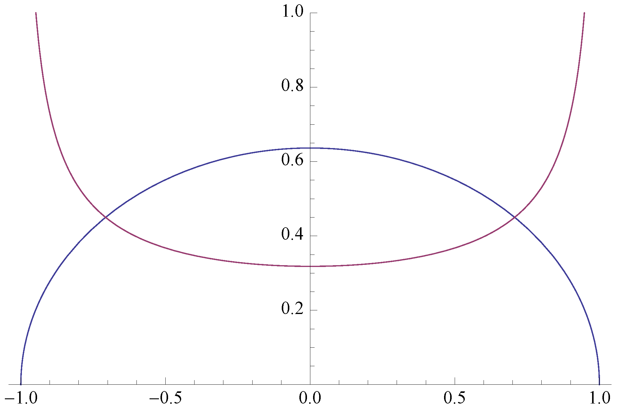
Answer: One can easily show that X has the “semi-circular” probability density function (pdf) given by
(See Figure 1.) By symmetry, Y has the same pdf as X.
Question 2. Let be a random vector uniformly distributed on the unit circle in . Find the marginal probability distributions of X and Y.
Answer: We can represent as where . It follows readily that X has pdf
(See Figure 1.) By symmetry, Y has the same pdf as X.
In both cases, the joint distribution of is circularly symmetric, that is, invariant under all orthogonal transformations of . A comparison of the shapes of the pdfs in Figure 1 suggest a third question:
Question 3. Does a circularly symmetric bivariate distribution with uniform marginals exist on ? If so, it determines a circular copula on , which is unique by Proposition 2.1. This also follows from uniqueness results for the Abel transform; see, e.g., Bracewell [6].
Answer: Optimistically, let’s seek an absolutely continuous solution. That is, we seek a bivariate pdf on of the form
such that the marginal pdf
is constant in x. Here g is a nonnegative function on that must satisfy
in order that (transform to polar coordinates: ).
To determine a suitable g, first set , then let to obtain
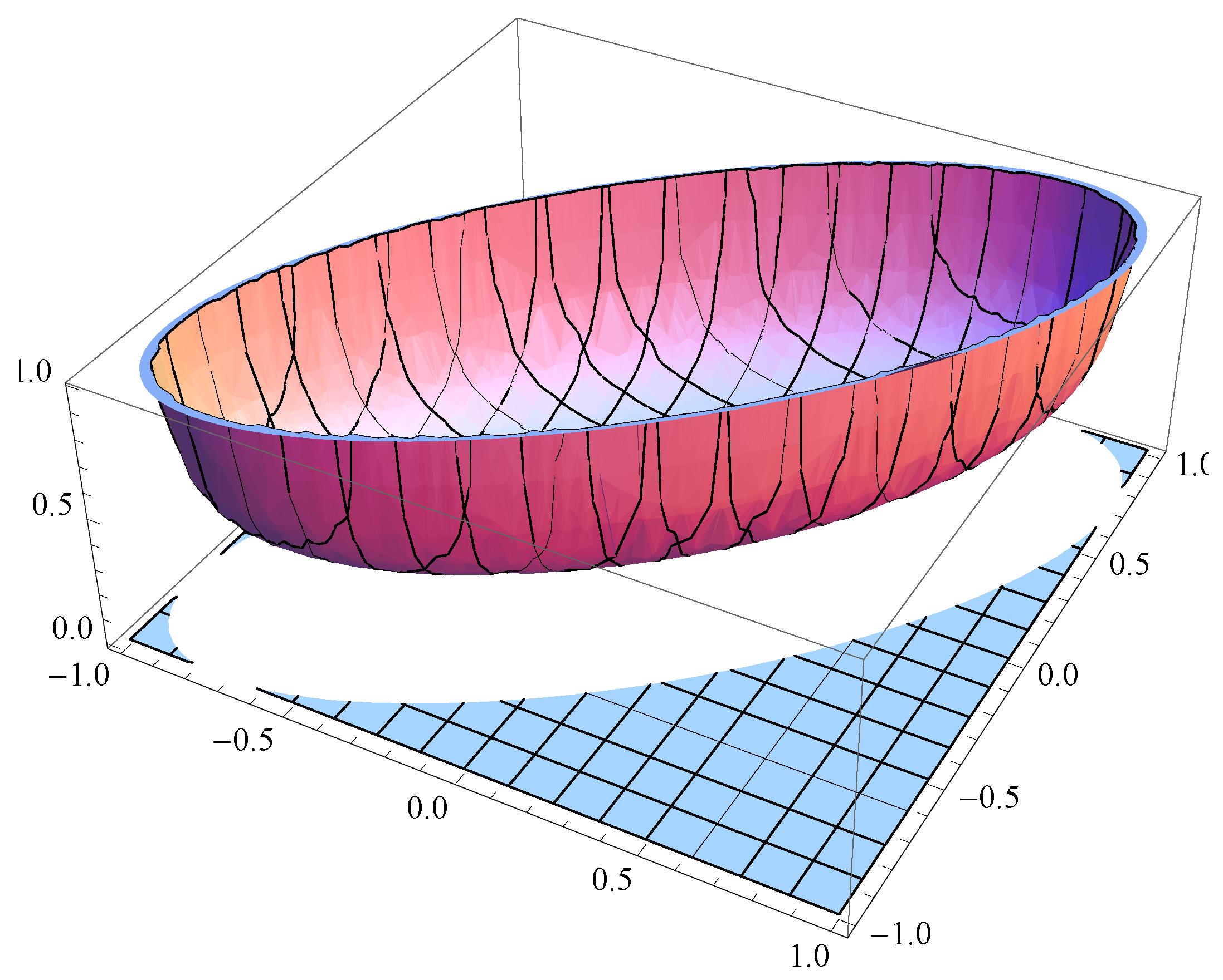
If we take then clearly does not depend on x, and choosing satisfies (5). Thus the bivariate pdf (see Figure 2)
determines a circularly symmetric bivariate distribution on and yields the desired circular copula.
Question 4. Having determined the unique circularly symmetric distribution (6) on with uniform marginals, what is the corresponding cdf , that is, what is the corresponding circular copula?
Answer (see Theorem 3.1): The circular symmetry of implies that its distribution is invariant under sign changes, i.e., . By the following lemma, the cdf on can be expressed in terms of , its truncation to the first quadrant:
for , and also in terms of the complementary cdf for . Because and has uniform marginals,
Lemma 3.1.
Let be a bivariate random vector on with uniform marginal distributions and sign-change invariance, i.e., . Then for ,
where if and .
Proof.
To obtain (9), consider four cases:
Case 1: . Because is sign-change invariant and has uniform marginals,
Case 2: . Similarly,
Case 3: . Similarly,
Case 4: . Similarly,
Thus, to determine the circular copula for the pdf (6), it suffices to determine the complementary cdf for and apply (10). Because when , we need only consider the case where .
However, we were unable to evaluate this integral directly.
Second approach: Fortunately, we have found a solution in the molecular biology and optics literatures, where the problem of finding the area of the intersection of two spherical caps on the unit sphere has been addressed. The following general result is due to Tovchigrechko and Vakser [7] and also appears in Oat and Sander [8].
Lemma 3.2.
This result can be applied to obtain our desired circular copula as follows.
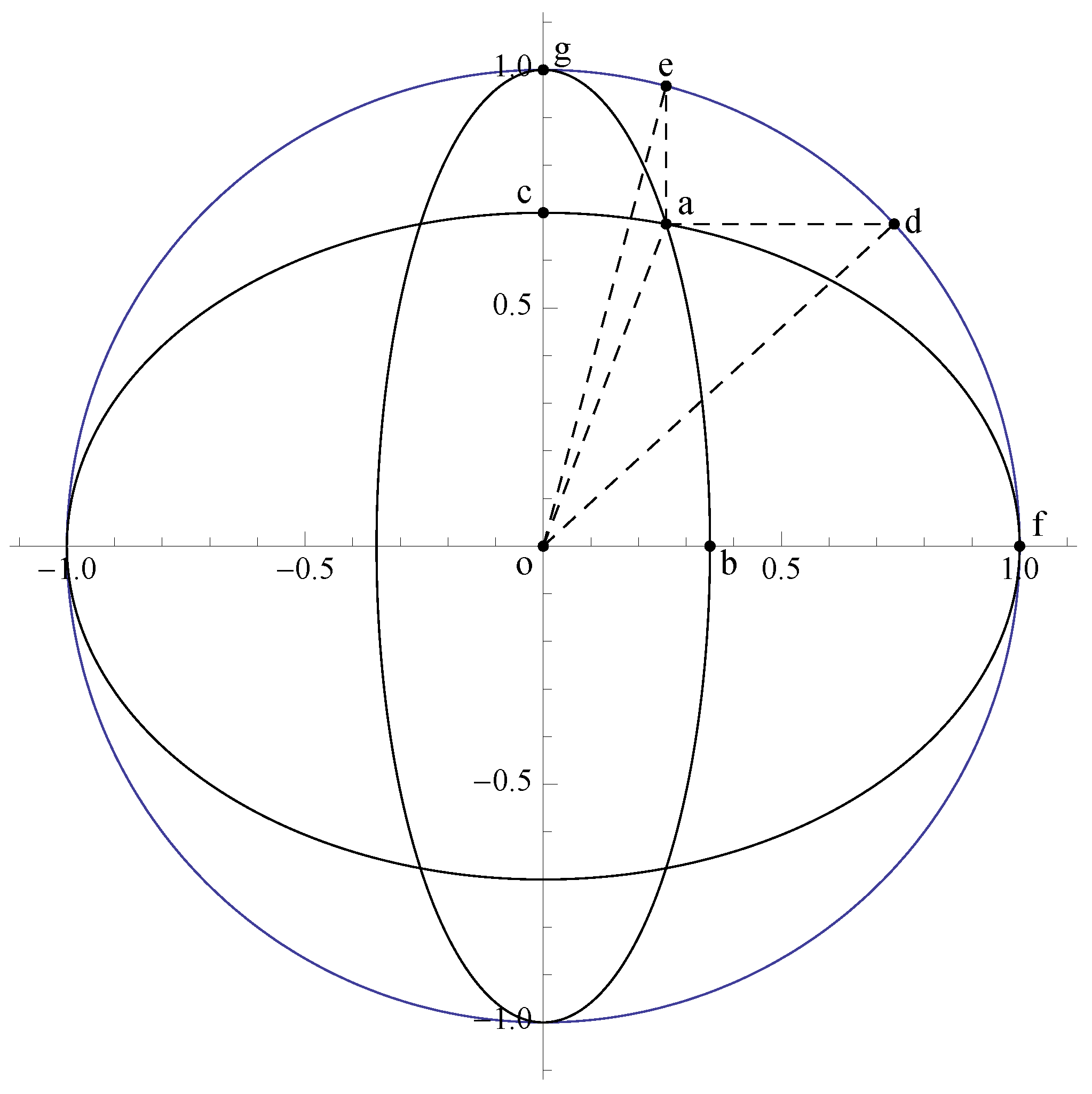
If is uniformly distributed on , then the event corresponds to the intersection of the two spherical caps and , so is given by the area of this intersection divided by the total area of , i.e., by . (See Figure 4 and Figure 5.) Also, the joint distribution of is circularly symmetric on the unit disk and has uniform marginals, so must be the unique such bivariate distribution, namely the distribution with pdf (6).
Thus, for and , our desired complementary cdf is given by
where for and ,
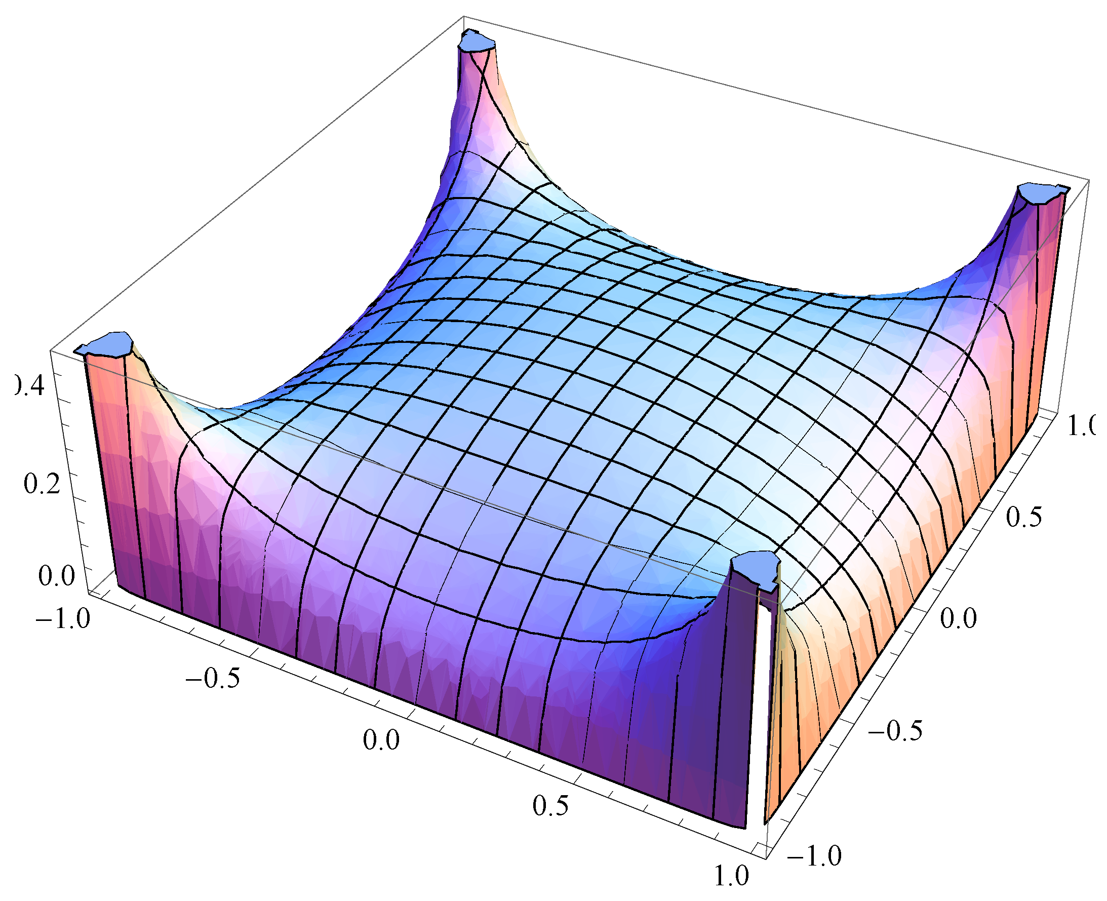
Theorem 3.1.
Proof.
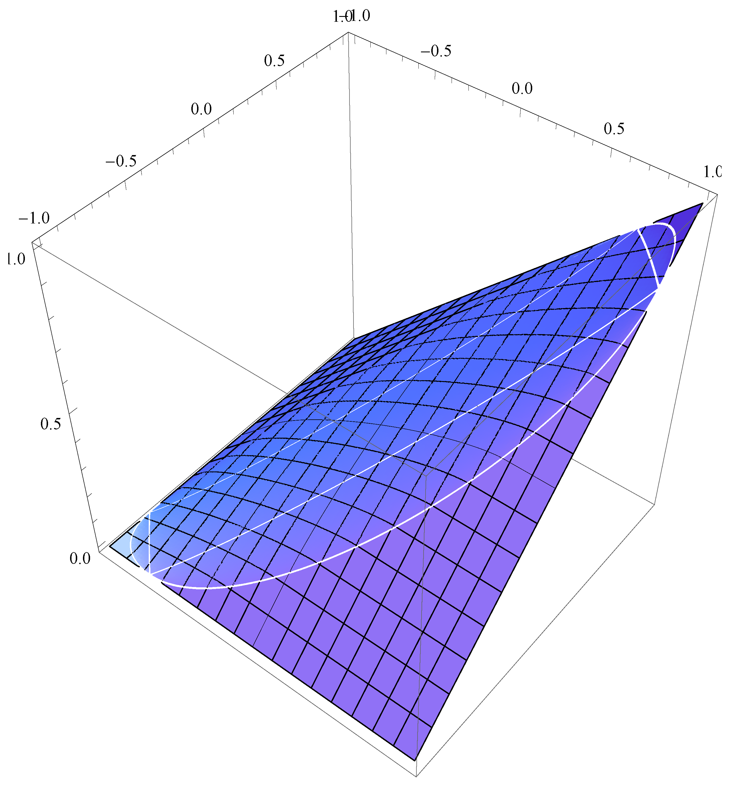
See Figure 6 for a plot of the resulting copula (on ).
4. The Trivariate Case: the Unique Spherical Copula
Question 5. Having determined the unique spherically symmetric distribution on with uniform marginals, namely, the uniform distribution on the unit sphere , what is the corresponding cdf on , i.e., the unique spherical copula?
Answer: As in Section 3, let be uniformly distributed on , so that . Again we first determine the complementary cdf for and , the intersection of the first octant of with the interior of . Here the event corresponds to the intersection of the three spherical caps , , and on , so is the area of this intersection divided by the total area of .
Recall that two approaches were proposed in Section 3 to obtain the area of the intersection of two circular caps and . The first approach led to the integral (11) that we were unable to evaluate explicitly, so we adopted a second approach based on the geometric Lemma 3.2 of Tovchigrechko and Vakser [7]. Andrey Tovchigrechko has kindly suggested a method for extending Lemma 3.2 to the case of three spherical caps in general position, which if carried out would yield an explicit expression for . However, we have found that because the axes of our three caps are mutually orthogonal, the two approaches just mentioned for the bivariate case can be combined to obtain directly for the trivariate case, as now described.
We begin by extending (11) to obtain an integral expression for when and . We require the fact that
Lemma 4.1.
If and , then
Because is exchangeable, (23) remains valid under any permutation of on the right-hand side.
As noted above, the integral in (23) appears difficult to evaluate explicitly but the following indirect argument succeeds. Recall from (11) and (15) that when and ,
where is given by (16). Because when and , it follows that
By (22), however,
so if we define by
for and , then
where is given by (16). Now (22) gives
so the above simplifies to
where
a symmetric function of . By (22), however,
and
so , hence identically in . Therefore we conclude that
for and .
We now apply (28) to obtain the cdf for all . For this, extend the definition of in (27) to all by means of (16) and (18).
Theorem 4.1.
The unique spherical copula on is given as follows:
for ,
Proof.
See [9]. □
5. A One-Parameter Family of Elliptical Copulas
Let in (6), the unique circularly symmetric distribution on the unit disk with uniform marginals. For any angle , consider the transformed variables
By the circular symmetry of , , so the random vector again generates a copula on the centered square . Denote the pdf and cdf of by and respectively. Then is a one-parameter family of elliptical copulas, so-called because the support of is the ellipse
(Note that .) From (29), the correlation coefficient of U and is given simply by
so indicates the degree of linear dependence between U and .
Proposition 5.1.
The pdf of is given by
Proof.
Thus the Jacobian of the transformation is , so from (6) we obtain
□
Figure 8 shows the density with .
To describe the family of elliptical copulas , we extend the definitions (16) and (18) as follows. First, for define
Next, extend the definition of to as follows (see Figure 9):
Note that (34) and (36) agree on , i.e., when . Also note that (36) reduces to in (18) when . The following lemma will be useful for the proof of Theorem 5.1.
Lemma 5.1.
Let be a bivariate random vector in with uniform marginals that satisfies . Then the cdf satisfies
Proof.
By the symmetry condition,
□
Theorem 5.1.
The cdf ≡ copula of is given by (see Figure 12)
Proof.
To find we again use the formula (12) for the area of the intersection of two spherical caps on . Here, unlike (14), the axes of the two caps are not necessarily perpendicular. The single formula (38) is obtained by considering the partition , where are defined in (36) and (see Figure 9)
Case 3: . Then , so by Lemma 5.1 and Case 2,
Case 4: . Then , so by Lemma 5.1 and Case 1, the argument for Case 3 applies verbatim.
Case 5: .
Case 6: .
Case 7: . Then , so by Lemma 5.1 and Case 6, the argument for Case 3 applies verbatim.
Case 8: . Then , so by Lemma 5.1 and Case 5, the argument for Case 3 applies verbatim. □
6. Copulas Derived from the Uniform Distribution on the Unit Ball
Up to now we have addressed the question of whether copulas can be generated by means of linear functions of a circularly symmetric or spherically symmetric random vector. Now we ask whether non-linear functions of such random vectors can generate copulas. We shall restrict attention to random vectors uniformly distributed over the unit ball and produce relatively simple non-linear functions that generate copulas on .
We begin with the bivariate case. Suppose that is distributed uniformly on the unit disk . Because
it follows that the random variables
satisfy
Thus, U and Y are independent, V and X are independent, and unconditionally,
so the joint distribution of generates a copula on the centered cube . Note that U and V are not linear functions of .
Question 6: Are U and V independent, and if not, what is the nature of their dependence?
Answer: Clearly U and V are uncorrelated, since and
all by the circular symmetry of . However, the joint pdf and cdf of derived below show that they are not independent.
Proposition 6.1.
The joint density of is given by (see Figure 13)
Proof.
This pdf is again obtained via the Jacobian method. It follows from (39) that
Substitution of the second expression for into the left side of the first relation and vice versa yields
so, since x and u (y and v) have the same signs by (39), we obtain
Thus
By symmetry it follows that the Jacobian is given by
and hence the determinant of J is given by
Because the pdf of is , the result (40) follows. □
For , , let and be the ellipses
The next lemma leads to the cdf corresponding to the pdf (40).
Lemma 6.1.
Proof.
Because is sign-change invariant and has uniform marginals, it follows from (7) and (9) in Lemma 3.1 and from (39) that for ,
The result now follows from Lemma 6.1. □
Remark:
The construction (39) extends readily to generate a copula on . For , for example, let be uniformly distributed on the unit ball and define
Then the marginal distributions of U, V, and W are each uniform so the cdf is a copula on . To find this copula one would need to determine , where now, for , , , and are the ellipsoids
Acknowledgements
We gratefully acknowledge several helpful suggestions by Ilya Vakser and Andrey Tovchigrechko.
References
- Nelsen, R.B. An Introduction to Copulas, 2nd ed.; Springer Series in Statistics; Springer: New York, NY, USA, 2006. [Google Scholar]
- Feller, W. An Introduction to Probability Theory and Its Applications, 2nd ed.; John Wiley & Sons Inc.: New York, NY, USA, 1971; Volume II. [Google Scholar]
- Arellano-Valle, R.B. On some characterizations of spherical distributions. Statist. Probab. Lett. 2001, 54, 227–232. [Google Scholar] [CrossRef]
- Schoenberg, I.J. Metric spaces and completely monotone functions. Ann. Math. 1938, 39, 811–841. [Google Scholar] [CrossRef]
- Cambanis, S.; Huang, S.; Simons, G. On the theory of elliptically contoured distributions. J. Multivar. Anal. 1981, 11, 368–385. [Google Scholar] [CrossRef]
- Bracewell, R.N. The Fourier Transform and Its Applications, 3rd ed.; McGraw-Hill Book Co.: New York, NY, USA, 1986. [Google Scholar]
- Tovchigrechko, A.; Vakser, I.A. How common is the funnel-like energy landscape in protein-protein interactions? Protein Sci. 2001, 10, 1572–1583. [Google Scholar] [CrossRef] [PubMed]
- Oat, C.; Sander, P.V. Ambient aperture lighting. In Proceedings of the 2007 Symposium on Interactive 3D Graphics, SI3D 2007, Seattle, WA, USA, 30 April–2 May 2007; Gooch, B., Sloan, P.P.J., Eds.; ACM: New York, NY, USA, 2007; pp. 61–64. [Google Scholar]
- Perlman, M.D.; Wellner, J.A. Squaring the Circle and Cubing the Sphere: Circular and Spherical Copulas; Technical Report 578; University of Washington, Department of Statistics: Seattle, WA, USA, 2010; Available at http://www.stat.washington.edu/research/reports/2011/tr578.pdf (accessed on 23 August 2011).
Figure 1.
The densities (3) (lower, blue) and (4) (upper, purple).

Figure 2.
Circularly symmetric bivariate density (6) on .
Figure 2.
Circularly symmetric bivariate density (6) on .

Figure 3.
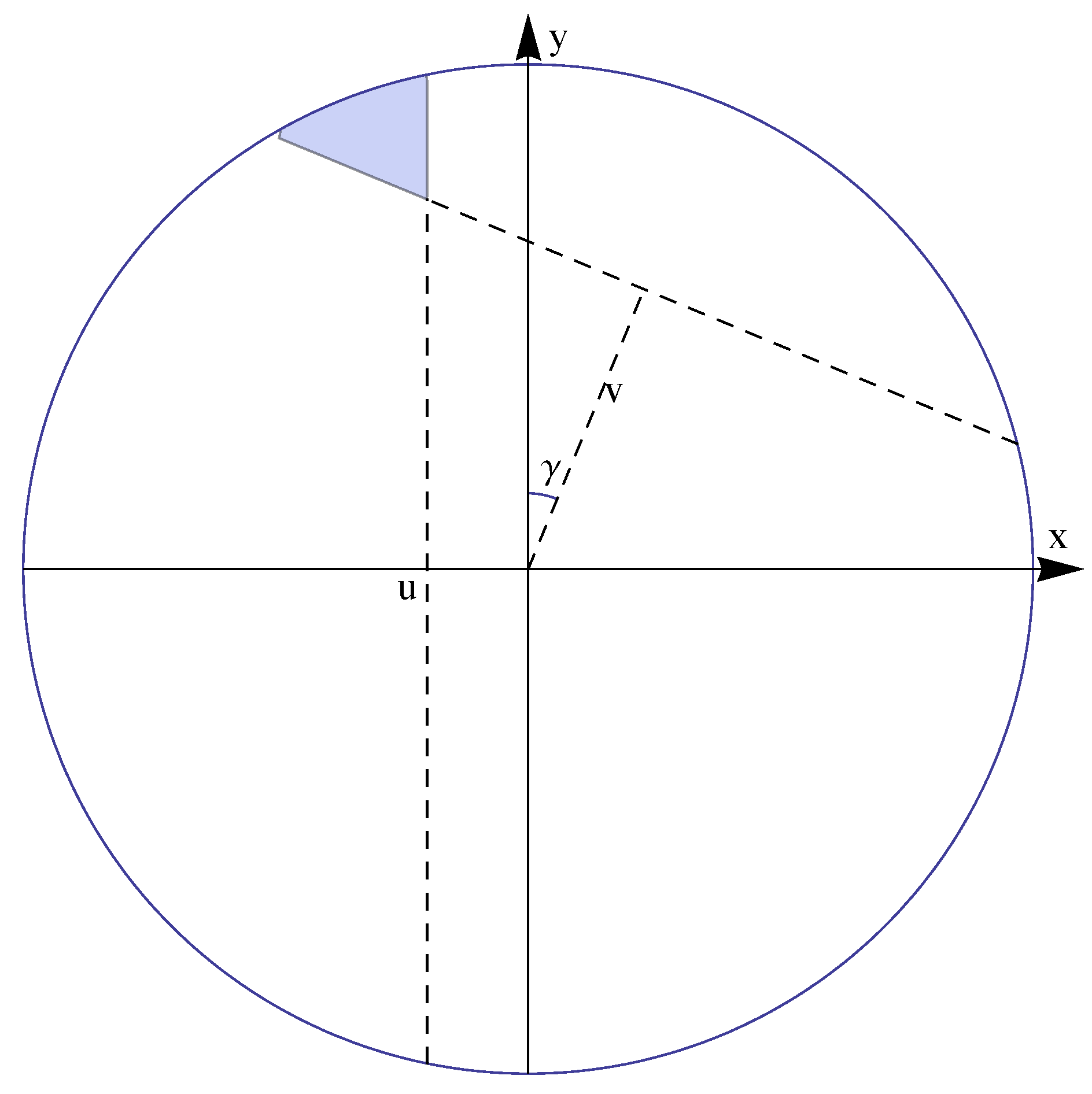
Region of integration, 2-dimensional case.

Figure 4.
Intersection of two spherical caps.

Figure 5.
Intersection of two spherical caps, circular representation (modified from Tovchigrechko and Vakser [7]).
Figure 5.
Intersection of two spherical caps, circular representation (modified from Tovchigrechko and Vakser [7]).

Figure 6.
The copula (17) in Theorem 3.1.
Figure 6.
The copula (17) in Theorem 3.1.

Figure 7.
Region of integration, 3-dimensional case, Lemma 4.1.

Figure 8.
The density in (32) (with ).
Figure 8.
The density in (32) (with ).

Figure 9.
Eight regions for an elliptical copula (with ).

Figure 10.
The region for Case 1 (with ).

Figure 11.
The region for Case 2 (with ).

Figure 12.
The copula in (38) (with ).
Figure 12.
The copula in (38) (with ).

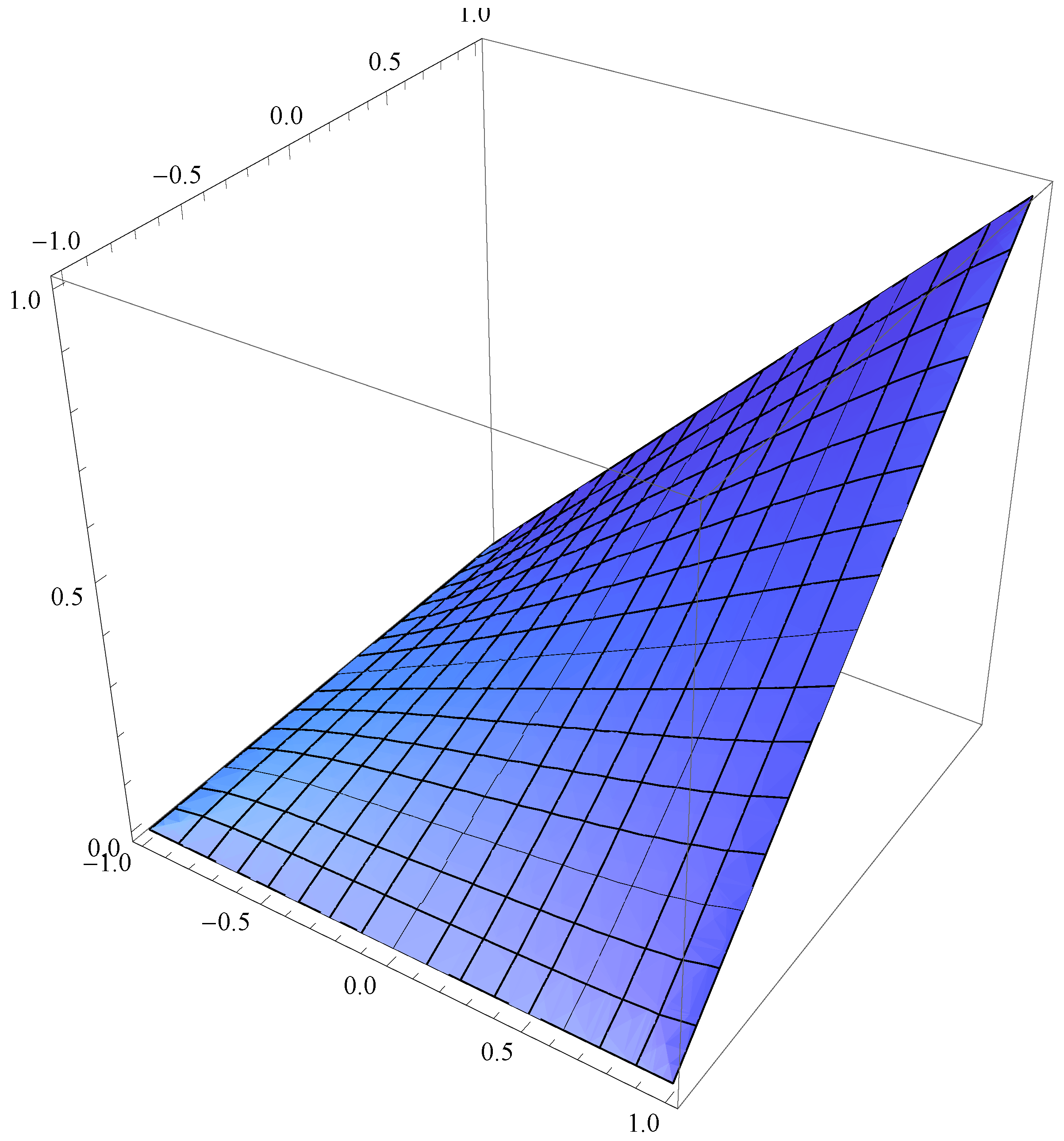
Figure 13.
Joint density of in (40).
Figure 13.
Joint density of in (40).

Figure 14.
Integration regions for Lemma 6.2.

Figure 15.
Nonlinear transformation copula in Theorem 6.1.

© 2011 by the authors; Licensee MDPI, Basel, Switzerland. This article is an open access article distributed under the terms and conditions of the Creative Commons Attribution (CC BY) license (http://creativecommons.org/licenses/by/3.0/).
Share and Cite
MDPI and ACS Style
Perlman, M.D.; Wellner, J.A. Squaring the Circle and Cubing the Sphere: Circular and Spherical Copulas. Symmetry 2011, 3, 574-599. https://doi.org/10.3390/sym3030574
AMA Style
Perlman MD, Wellner JA. Squaring the Circle and Cubing the Sphere: Circular and Spherical Copulas. Symmetry. 2011; 3(3):574-599. https://doi.org/10.3390/sym3030574
Chicago/Turabian StylePerlman, Michael D., and Jon A. Wellner. 2011. "Squaring the Circle and Cubing the Sphere: Circular and Spherical Copulas" Symmetry 3, no. 3: 574-599. https://doi.org/10.3390/sym3030574