Knot Quandaries Quelled by Quandles

This column will introduce the more recent theory of quandles, an elementary algebraic structure that may be associated to a knot...

Introduction

Knottedness is all around us: our earphones get knotted; we grudgingly spend time untangling the garden hose in the spring; DNA molecules are knotted in the nuclei of our cells.

Sailors and rock climbers know there are different types of knots having different properties. Mathematics, in fact, gives a language and tools for describing knots and their properties.

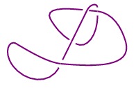
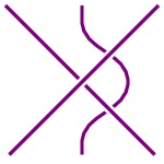
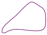
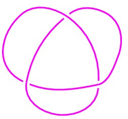
The central problem of knot theory is to determine when two knots are the same. For instance, if you construct the knot on the left by connecting one end of a garden hose to the other, can you move it around, without disconnecting it, to make it look like the one on the right?

 

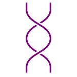
Though simple to ask, this question can be devilishly difficult to answer because there is so much flexibility in how we can move knots. We may intuitively feel that two knots, such as the ones shown below, are different, but how can we be sure that a way of moving one into the other just hasn't eluded us.

 

To get around this flexibility, knot theorists frequently associate some additional structure to a knot that does not depend on how we look at it. An early example is the Alexander polynomial, which associates to a knot $K$ a polynomial $\Delta_K(t)$. If two knots $K_1$ and $K_2$ have distinct Alexander polynomials, we can be sure that the knots are themselves distinct. We call such an association a knot invariant.

This column will introduce the more recent theory of quandles, an elementary algebraic structure that may be associated to a knot. When the quandles associated to two knots are distinct, we know that the knots are distinct.

While there are many new and powerful knot invariants created with relatively sophisticated mathematical tools, the theory of quandles is accessible to undergraduate mathematics students and produces invariants that are easily computable. In this way, we may observe a powerful connection between topology and algebra.

Knot diagrams and Reidemeister moves

As mentioned above, knots are complicated because there are so many ways in which we can move them around. Fortunately, there is a wonderful theorem that tells us when two illustrations of knots depict the same knot.

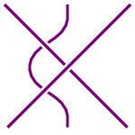
A figure like the one below is meant to illustrate a knot drawn in three dimensions. Let's begin, however, by viewing it simply as a two-dimensional figure consisting of arcs and some crossings. Such a figure is called a knot diagram.

 

There are three simple ways in which we may modify knot diagrams without changing the three-dimensional knot that they represent. These are known as Reidemeister moves.

Move I:		$\Longleftrightarrow$
Move II:		$\Longleftrightarrow$
Move III:		$\Longleftrightarrow$

In the 1920's, Reidemeister proved this useful theorem: Given two knot diagrams representing the same knot, there is a sequence of Reidemeister moves transforming one diagram into the other.

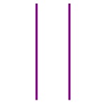
For instance, if you study the two knot diagrams below, you may sense they represent the same knot, which we call the unknot.

 

Here is a sequence of Reidemeister moves, read left to right and then top to bottom, transforming one diagram into the other.

 

Reidemeister's theorem is especially useful for creating knot invariants; if we find a way to associate some structure to a knot diagram and show that this structure does not change when we apply Reidemeister moves, then we have created a knot invariant. Let's illustrate this by looking at the colorability of knots.

Comments?

Fox's three-colorability

Fox introduced a simple knot invariant in the 1950's by coloring the arcs in a knot diagram. More specificaly, we ask whether we can color the arcs in a knot diagram using three colors in such a way that when three arcs meet at a crossing, the three arcs have either the same color or three distinct colors. These two possibilities are shown below.

 

A coloring of a knot diagram satisfying this condition is called a three-coloring.

 

It may appear that a three-coloring depends on a particular knot diagram rather than the underlying knot. However, the Reidemeister moves allow us to show that a three-coloring of one knot diagram produces a unique three-coloring of every knot diagram of the same knot. There are several posssibilities to check, a few of which are shown below.

Move I:		$\Longleftrightarrow$
Move II:		$\Longleftrightarrow$
Move III:		$\Longleftrightarrow$

In this way, a three-coloring of a knot diagram may be thought of as a three-coloring of the knot. A simple knot invariant is then given by counting the number of three-colorings of a knot.

Of course, every knot has three trivial three-colorings in which every arc is given the same color. A more interesting question asks whether a knot admits any nontrivial three-colorings as illustrated on the left.

 

Naturally, the unknot, which may be represented by a knot diagram containing a single arc, admits no nontrivial three-coloring. This allows us to conclude the knot on the left is not equivalent to the unknot.

 

You may wish to check that the trefoil knot, shown on the right, has nine three-colorings. Three of these are trivial; once you have found one nontrivial three-coloring, you may find five more by permuting the colors. Therefore, the trefoil knot is not equivalent to the unknot.

However, the Figure 8 knot, shown on the right, admits no nontrivial three-colorings. This does not imply that the Figure 8 knot is equivalent to the unknot. Instead, it only implies that counting three-colorings does not give us enough information to distinguish the Figure 8 from the unknot.

 

Counting three-colorings produces a rather crude knot invariant as it is not capable of distinguishing many pairs of distinct knots. However, it points the way toward the creation of more powerful invariants.

Comments?

Using linear algebra to find three-colorings

Before going on, let's reframe the problem of counting three-colorings using linear algebra.

To do this, we will associate to each of our three colors an element of the set $\{0,1,2\}$, which we think of as ${\Bbb Z}_3$, the set of mod 3 congruence classes. A coloring of a knot diagram then corresponds to labeling each arc in the diagram with an element of this field. More specificaly, we associate to the $i^{th}$ arc an element $x_i\in\{0,1,2\}$.

For instance, the knot diagram we considered earlier leads to the labeling

 

In ${\Bbb Z}_3$, we obtain a solution to the equation $a+b+c=0$ when either $a=b=c$ or $a$, $b$, and $c$ are pairwise distinct. This is precisely the condition that must hold at each crossing to obtain a three-coloring. Therefore, a three-coloring of the knot is described by a solution to the equations: \[ \begin{align} x_1 + x_6 + x_7 & = 0 \\ x_1 + x_2 + x_7 & = 0 \\ x_2 + x_4 + x_7 & = 0 \\ x_2 + x_3 + x_4 & = 0 \\ x_2 + x_3 + x_5 & = 0 \\ x_3 + x_5 + x_6 & = 0 \\ x_4 + x_5 + x_8 & = 0 \\ x_1 + x_5 + x_8 & = 0 \end{align} \]

The coefficient matrix for this set of equations (below, left) has the following reduced row echelon form (below, right): \[ \left[ \begin{array}{cccccccc} 1 & 0 & 0 & 0 & 0 & 1 & 1 & 0 \\ 1 & 1 & 0 & 0 & 0 & 0 & 1 & 0 \\ 0 & 1 & 0 & 1 & 0 & 0 & 1 & 0 \\ 0 & 1 & 1 & 1 & 0 & 0 & 0 & 0 \\ 0 & 1 & 1 & 0 & 1 & 0 & 0 & 0 \\ 0 & 0 & 1 & 0 & 1 & 1 & 0 & 0 \\ 0 & 0 & 0 & 1 & 1 & 0 & 0 & 1 \\ 1 & 0 & 0 & 0 & 1 & 0 & 0 & 1 \\ \end{array} \right] \sim \left[ \begin{array}{cccccccc} 1 & 0 & 0 & 0 & 0 & 0 & 0 & 2 \\ 0 & 1 & 0 & 0 & 0 & 0 & 1 & 1 \\ 0 & 0 & 1 & 0 & 0 & 0 & 2 & 0 \\ 0 & 0 & 0 & 1 & 0 & 0 & 0 & 2 \\ 0 & 0 & 0 & 0 & 1 & 0 & 0 & 2 \\ 0 & 0 & 0 & 0 & 0 & 1 & 1 & 1 \\ 0 & 0 & 0 & 0 & 0 & 0 & 0 & 0 \\ 0 & 0 & 0 & 0 & 0 & 0 & 0 & 0 \\ \end{array} \right] \]

This shows that the solution space is a two-dimensional subspace of ${\Bbb Z}_3^8$, which therefore has $3^2=9$ elements. Hence, there are nine three-colorings, three of which are trivial and six of which are obtained by permuting the colors in this nontrivial three-coloring.

 

As mentioned above, counting three-colorings is not a particularly strong knot invariant. It does, however, point to an important connection between algebra and the topology of knots, a connection that deepens, as we'll see, with the introduction of quandles.

Quandles

Our discussion of three-colorings naturally led to algebraic considerations using the field ${\Bbb Z}_3$. We will now introduce a new algebraic structure, called a quandle, which is somewhat similar to a group and which has properties that make it ideally suited to studying knots.

Before defining a quandle, let's consider labelings of knot diagrams in light of the Reidemeister moves. Notice that we will be working with oriented knots; that is, knots along which we travel in a preferred direction.

 

The crossings of an oriented knot come in two types, which are labeled as +1 and -1.

 

+1	-1

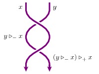
Let's think of a knot diagram as a collection of arcs $A=\{a, b, c, \ldots\}$ together with a collection of crossings. We will record the relation between the arcs at a crossing using two binary operations as shown below.

 

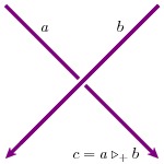
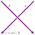
That is, if arc $a$ crosses under $b$ in a +1 crossing, it becomes arc $c = a \triangleright_+ b$. Similarly, if $a$ crosses under $b$ in a -1 crossing, it becomes $c=a\triangleright_-b$. In this way, the operations $\triangleright_+$ and $\triangleright_-$ record the relationships between the arcs at the crossings.

Since we hope to create knot invariants, we would like these operations to be consistent when a Reidemeister move is applied to a knot diagram. We will study each move in its turn and use the results to motivate the definition of a quandle.

• Move I:

   

  

  This shows that we should require that $x\triangleright_+ x = x \triangleright_- x = x$.

   

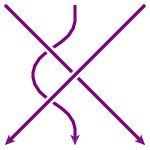
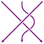
• Move II:

   

  

  This shows that $$ (y\triangleright_- x) \triangleright_+ x = y = (y\triangleright_+ x) \triangleright_- x. $$

  In other words, the operations $\triangleright_+$ and $\triangleright_-$ are inverses of one another. Consequently, we will consider a single operation $\triangleright = \triangleright_+$ with inverse $\triangleright^{-1} = \triangleright_-$.

   

• Move III:

   

  
  
  

  With a little bit of work, this move leads to the following distributivity relationship: $$ (x\triangleright y)\triangleright z = (x\triangleright z) \triangleright (y\triangleright z).$$

Motivated by these observations, we define a quandle to be a set $X$ with a binary operation $\triangleright$ such that:

1. For all $x\in X$, we have $x\triangleright x = x$.

    

2. Given $y\in X$, we may define the function $\beta_y:X\to X$ by $\beta_y(x) = x\triangleright y$. For all $y$, this function is invertible.

    

3. For all $x,y,z\in X$, $(x\triangleright y)\triangleright z = (x\triangleright z)\triangleright (y\triangleright z)$.

This definition may remind you of the definition of a group, which also involves a set and a binary operation satisfying three properties. A quandle's binary operation, however, satisfies a different set of properties, which are chosen to mimic the relationship between the arcs in a knot diagram.

Let's look at some examples of quandles.

1. Groups give rise to quandles: Suppose that $G$ is a group. Defining the operation $\triangleright$ by $g\triangleright h = h^{-1} g h$ makes the set $G$ into a quandle. This is easy to see:

   1. If $g\in G$, then $g\triangleright g = g^{-1}gg = g$.

   2. If $h\in G$, then $\beta_h:G\to G$ is defined by $\beta_h(g) = h^{-1}gh$. The inverse of $\beta_h$ is $\beta_{h^{-1}}$.

   3. If $g,h, k\in G$, then \[ \begin{align} (g\triangleright h)\triangleright k = & (h^{-1}gh)\triangleright k \\ = & k^{-1}h^{-1}ghk \\ = & (k^{-1}h^{-1}k)(k^{-1}gk)(k^{-1}hk) \\ = & (k^{-1}hk)^{-1}( k^{-1}gk)(k^{-1}hk) \\ = & (k^{-1}gk) \triangleright (k^{-1}hk) \\ = & (g\triangleright k) \triangleright (h\triangleright k) \end{align} \]

    

2. Alexander quandles: Consider the set of mod $n$ congruence classes ${\Bbb Z}_n$, and choose an integer $t$ relatively prime to $n$. This implies that $t$ has a multiplicative inverse $t^{-1}$ in ${\Bbb Z}_n$.

   We obtain the quandle $\Lambda_{n,t}$ with underlying set ${\Bbb Z}_n$ by defining $$x\triangleright y = tx + (1-t)y.$$

   It is easy to see this forms a quandle:

   1. $x\triangleright x = tx + (1-t)x = x$.
   2. If $\beta_y(x) = z = x\triangleright y = tx + (1-t)y$, then $\beta_y^{-1}(z) = x = t^{-1}z + (1-t^{-1}) y$.
   3. Similarly, a straightforward computation verifies that $(x\triangleright y)\triangleright z = (x\triangleright z)\triangleright (y\triangleright z)$.

   For example, if we choose $n=3$ and $t=2$, then $x\triangleright y = 2x + (1-2)y = 2x + 2y$. We will soon see that this quandle, $\Lambda_{3,2}$, helps describe three-colorings of a knot.

   More generally, if $V$ is a vector space and $T:V\to V$ an invertible linear transformation, then $V$ becomes an Alexander quandle under the operation $x\triangleright y = Tx+(I-T)y$.

Comments?

Knot invariants from quandles

Earlier we created an invariant of knots by coloring the arcs in a knot diagram with one of three colors. We will now create invariants by "coloring" the arcs with elements of a quandle.

Given a knot diagram for a knot $K$ and a quandle $Q$, we form a $Q$-coloring of $K$ by labeling each arc in the diagram with an element of $Q$. At each crossing, we require that the labels associated to the arcs meeting at that crossing be related by the quandle operation $\triangleright$.

More specifically, we think of "coloring" the arcs in a knot diagram for $K$ with elements of $Q$ by labeling each arc $a_i$ with an element $x_i\in Q$. If a crossing gives the relationship $a_i\triangleright a_j = a_k$, then we require that $x_i\triangleright x_j=x_k$. Such a coloring is called a $Q$-coloring of the knot $K$.

For instance, consider the Alexander quandle $\Lambda_{3,2}$ and suppose $K$ is a knot with a knot diagram having arcs $a_1, a_2, \ldots a_n$. We label each arc $a_i$ with an element $x_i$ of $\Lambda_{3,2} = \{0,1,2\}$ just as we did when we created three-colorings.

Suppose that a crossing in the knot diagram leads to the relationship $a_i\triangleright a_j = a_k$. We require that the associated labels satisfy $x_i\triangleright x_j = x_k= 2x_i + 2x_j = -x_i - x_j$, or equivalently $x_i + x_j + x_k = 0$. This is precisely the condition that guaranteed a three-coloring of the knot.

Therefore, there is a 1-1 correspondence between three-colorings of the knot $K$ and $\Lambda_{3,2}$-colorings.

More generally, if $Q=\Lambda_{n,t}$, we assign to each arc $a_i$ an element $x_i\in \Lambda_{n,t}$ and require $x_i\triangleright x_j = tx_i + (1-t)x_j = x_k$. In other words, we obtain a system of equations, one for each crossing: $$ tx_i + (1-t)x_j - x_k = 0. $$

As this only requires us to solve a system of linear equations, it is easy to compute the number of $\Lambda_{n,t}$-colorings of a knot diagram.

In spite of the fact that a coloring is defined in terms of a knot diagram, counting quandles colorings produces a knot invariant. This is because a coloring of one knot diagram produces a unique coloring of any other knot diagram of the same knot.

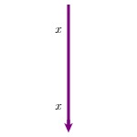
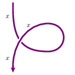
To see this, remember that knot diagrams of the same knot are related by a sequence of Reidemeister moves and that for each of the three moves, we understand how the arcs and crossings change. For instance, suppose that we perform Reidemeister move I.

 

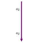
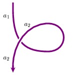
Before the move, we have a single arc $a_2$, as shown on the left, that is assigned the color $x_2$. After the move, we have two arcs $a_1$ and $a_2$; color $a_1$ with the same color as $a_2$ so that $x_1=x_2$. At the crossing created by the move, we have $a_1\triangleright a_2 = a_2$. We just need to check that $x_1\triangleright x_2 = x_2$, which naturally follows from the quandle condition $$ x_1\triangleright x_2 = x_2\triangleright x_2 = x_2. $$

Similar arguments apply to the other Reidemeister moves.

Remember that every knot admits trivial three-colorings. In the same way, we may color every arc in a knot diagram with the same element of a quandle $Q$. Because of the quandle relation $x\triangleright x = x$, this produces a trivial $Q$-coloring of the knot.

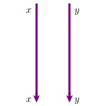
As an example, consider the two knots shown below:

 

$K_1=8_{11}$	$K_2=10_{18}$

Both knots have only trivial three-colorings. However, they may be distinguished by counting colorings by $\Lambda_{5,4}$; the knot $K_1$ admits only trivial $\Lambda_{5,4}$-colorings while $K_2$ has a nontrivial $\Lambda_{5,4}$-coloring.

The fundamental quandle of a knot

Every oriented knot $K$ has a quandle $Q_K$, called the fundamental quandle of $K$, that is naturally associated to it.

Begin with a knot diagram representing $K$. Ideally, the underlying set $Q_K$ would be the set of arcs in the knot diagram with $\triangleright$ recording the relationship between arcs that meet at a crossing. However, $x\triangleright y$ will not be defined if the arcs $x$ and $y$ do not meet at a crossing. In this case, we simply add a new element $x\triangleright y$ to the set $Q_K$ and continue to do so as needed.

For example, if $x$, $y$, and $z$ are arcs in the knot diagram, then $x\triangleright \big((y\triangleright x)\triangleright z\big)$ is an element of $Q_K$. Typically speaking, most of the elements in $Q_K$ are not arcs in the knot diagram.

Because the three conditions defining quandles were motivated by the effect of the three Reidemeister moves on the operator $\triangleright$, the quandle $Q_K$ is unchanged when the knot diagram is changed by a Reidemeister move. Therefore, $Q_K$ depends only on the underlying oriented knot $K$. The fundamental quandle also has a geometric interpretation in terms of homotopy classes of certain paths in the knot's complement.

As an algebraic object, we may consider homomorphisms between quandles. For instance, suppose that $Q$ and $Q'$ are quandles. A quandle homomorphism is a map $f:Q\to Q'$ that respects the $\triangleright$ operations in the sense that $f(q_1\triangleright q_2) = f(q_1)\triangleright f(q_2)$.

Notice that a $Q$-coloring of a knot $K$ is equivalent to a homomorphism $f:Q_K \to Q$. For instance, if an arc $a_i$ is labeled by $x_i$ in a $Q$-coloring, then define $f(a_i) = x_i$. The requirement that $a_i\triangleright a_j = a_k$ implies $x_i\triangleright x_j = x_k$ means that $f$ respects the $\triangleright$ operations.

Quandles $Q$ and $Q'$ are isomorphic if there is a bijective homomorphism $f:Q\to Q'$. We think of isomorphic quandles as being equivalent.

Now, the fundamental quandle of a knot is itself a knot invariant. That is, if $K$ and $K'$ are equivalent knots, then $Q_K$ and $Q_{K'}$ are isomorphic quandles.

It turns out that the fundamental quandle is an excellent knot invariant. In his original paper, Joyce proved that, up to the orientation of the knot, if $Q_K$ and $Q_{K'}$ are isomorphic quandles, then $K$ and $K'$ are equivalent knots. In other words, the fundamental quandle is really the best possible invariant as two different knots can never have the same fundamental quandle.

The problem, however, is that it is very difficult to determine whether the fundamental quandles of two knots are isomorphic. Counting quandle colorings is, as we have seen, much more practical since we can sometimes reduce the problem to that of solving a system of linear equations.

While we considered a simple class of quandles $\Lambda_{n,t}$ above, there are many other types of quandles we could use for coloring knots in the hope of distinguishing knots from one another. Given two knots $K_1$ and $K_2$, we may try to find a quandle $Q$ whose structure mimics some feature we see in $Q_{K_1}$ but that is not readily apparent in $Q_{K_2}$. In this case, counting $Q$-quandle colorings can give a computable means of checking that $Q_{K_1}$ and $Q_{K_2}$ are not equivalent quandles and that, hence, $K_1$ and $K_2$ are not equivalent.

Comments?

Summary

Quandles, which seem to have independently appeared at various times in the mathematical literature, form one of a collection of algebraic structures that are helpful in the study of knots. More familiar may be the fundamental group of a knot.

In 1942, Takasaki introduced a special type of quandle, which he called a kei, that is essentially a quandle in which the second condition is replaced by $(x\triangleright y)\triangleright y = x$; that is, $\triangleright$ is its own inverse.

Conway and Wraith introduced a similar structure known as a wrack in the 1950s before Joyce and Matveev, working independently, introduced what we have called quandles, following Joyce's terminology.

What I have written here is, in some sense, just the tip of the iceberg. Some readers may sense that the Alexander polynomial is lurking somewhere nearby and indeed it is. Now that we have the quandle's algebraic structure, we may start to play more sophisticated algebraic games in an effort to create more powerful knot invariants. In fact, there is a cohomology theory for quandles that has been used to obtain new results about knotted surfaces in 4-space.

Aside from describing some interesting mathematical ideas, my intention in writing this column has been to give an introduction to the subject of knot invariants that is hopefully accessible to undergraduates. A traditional undergraduate curriculum often leads students to see mathematics as a collection of disparate subjects, such as differential equations, algebra, topology, geometry. Quandles break through this seeming compartmentalization by showing how topological relationships may be naturally encoded in an algebraic structure, providing powerful tools for drawing topological conclusions that may be otherwise difficult to reach.

References

• Mohamed Elhamdadi and Sam Nelson. Quandles: An Introduction to the Algebra of Knots. American Mathematical Society. 2015.
  
  This book is a good introduction to quandles, and other algebraic structures associated with knots, geared toward an undergraduate audience.


• David Joyce. A classifying invariant of knots, the knot quandle. Journal of Pure and Applied Algebra 23, pp. 37-65, 1982.
   
• Sergei Matveev. Distributive groupoids in knot theory. Matematicheskii Sbornik 47(1), pp. 78-88, 1984.
   
• Masahico Saito and Chad Smudde. Quandle Cocycle Knot Invariants. A site aimed at about the same level as this article that further develops the algebra of quandles.
   
• Dale Rolfsen. Knots and Links. Publish or Perish. 1976.
   
• Louis Kauffman. Knots and Physics. World Scientific Publishing Company. 1991.