Building Trees for Biologists
Here I will look at some of the contributions that mathematics has made relatively recently to genetics/genomics and how mathematics grew as a consequence of attempts to model genetics/genomics problems using mathematical tools. ...
 Joseph Malkevitch
York College (CUNY)
Email Joseph Malkevitch
Introduction
Mathematics has always been a valuable tool for subjects such as physics, chemistry, and engineering. By comparison it has only been more recently that mathematics has proved to be as illuminating for biology. Examples abound of the way that mathematics and biology are cross-fertilizing each other, ranging from new approaches to finding the distance between two objects of interest (DNA sequences or ancestral trees), or studying the working of neurons or cells. However, there was a small section of biology that mathematics has had longer involvement with and success in. This is the area of genetics. While in some ways genomics and mathematical contributions to computational biology may overshadow this earlier work, it is still the case that methods and ideas developed in "classical" mathematical genetics continue to find applications even now. Some of these classical results are sometimes placed within the domain of population genetics.
Here I will look at some of the contributions that mathematics has made relatively recently to genetics/genomics and how mathematics grew as a consequence of attempts to model genetics/genomics problems using mathematical tools.
The idea that species evolve certainly had roots before Charles Darwin (1809-1882) but his book On the Origin of Species from 1859 was a landmark in intellectual history. Darwin was a great observer of nature and he extrapolated from his observations of the natural world both within his homeland England and on his travels (voyage of the Beagle). However, Darwin made limited use of mathematics in his work. He wrote: “I have deeply regretted that I did not proceed far enough at least to understand something of the great leading principles of mathematics; for men thus endowed seem to have an extra sense.” Many parts of mathematics have been brought to bear on understanding genetics and the genome with goals ranging from increasing the yields of crops, keeping livestock healthier, developing new drugs, finding ways to cure inherited diseases, and getting a basic understanding of the history of life on Earth.

Figure 1 (Photo of Charles Darwin; courtesy of Wikipedia.)
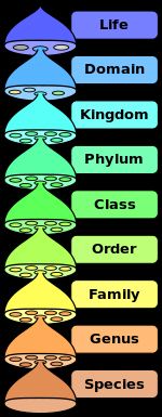
A basic tenet of evolution is that the species we see today are descended from species that existed in the past and any particular species alive today has origins in such past species. To understand the complexity of living things, scholars developed a classification system for living things that went from the specific to the general. Many scholars contributed to the taxonomy (classification) terms used today but here is a current version:
Figure 2 (Diagram of the hierarchy of life forms, courtesy of Wikipedia.)
Thus, there are many species within a particular genus, and American textbooks usually assert there are 6 kingdoms, but British books often use 5 kingdoms, and when the names in the two systems are lumped we get: Animalia, Plantae, Fungi, Protista, Archaea/Archaeabacteria, Bacteria/Eubacteria and Monera. At all levels of the classification system there are controversies. For a long time there was thought to be only one species of giraffe but recently it has been argued that giraffe belong to four different species. The basic notion of a species is that different species can't have reproducing offspring. However, the reality, as is typical in the sciences, is more complex. In reality, what can happen and in many cases did happen in the wild in the past was that different "species" did mate; the phenomenon is known as "hybridization." The hybrids sometimes may have become isolated, leading to a new species, or they may have become "integrated" via mating with one or both of the species that gave rise to the hybrids. In modern times, two different hybrids are, for example, ligers (lion father; tiger mother) and tigons (tiger father; lion mother).

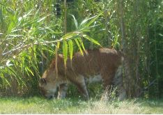
Figure 3 (Ligers (top) and tigon (bottom), courtesy of Wikipedia.)
Often hybrid males are not able to reproduce though females can, but it appears that sometimes the male hybrids can have progeny. Recently quite a bit of attention has been paid to the fact that there seems to be DNA evidence that the two hominid "species" homo sapiens and Neanderthal interbred and the genetic legacy of this can be found in the genomes of modern homo sapiens.
We will return to classification issues shortly but first let us take a "detour" to put in perspective how the taxonomy issues of what is being investigated today build on our biological insights since Darwin.
When early naturalists tried to tell which bird species were alike (or different) they would typically use things like size of the bird, size and shape of bird beaks, etc. to group the birds. However, with the advent of modern biology's discovery of the role of DNA in genetics, new ways were developed to tell which species were close and which ones were far apart.
There are different approaches to looking at what is the makeup of the genetic material of a species. One can think of the genome of species X as just one long DNA string, as a collection of chromosomes, or as a collection of genes that are located at various places on the chromosomes. When we speak of comparing the genome, say, of a chimp with that of a human there are already complications. Humans have 46 chromosomes (23 pairs) while chimps have 48 chromosomes (24 pairs) though it is thought that we have a good understanding of how these chromosomes match up and there are two pairs of chromosomes of the chimp that seem to "match up" with one pair of human chromosomes. Recall that for most pairs of chromosomes, an individual is made up of one chromosome of a pair from the father and one chromosome of a pair from the mother. One complication is the issue of the sex (female or male) of a human (or chimp). Of the 23 pairs of human chromosomes, 22 are known as autosomes and there is one pair known as sex chromosomes. Usually, the sex chromosomes are known as X and Y chromosomes. Women have two X chromosomes and men have one X chromosome and one Y chromosome. (But as is often the case the usual is not the full story.) Girls get one X chromosome from their dad and one from their mom. Boys must have gotten the Y chromosome from their dad (and not his X chromosome) and one of the two X chromosomes from their mom.
Typically, one looks inside the nucleus of a cell for the genetic material, where one finds the chromosomes, but there is also genetic material in the mitochondria, which are structures (organelles) found within most cells and which are involved with the energy needs of the cell. The genetic material in the mitochondria in humans is only inherited from one's mother. In some ways tracking genetic material in the mitochondria simplifies the "mechanics" of determining inheritance of traits but the price is that any individual's full genetic endowment is a mixture of what one gets from both of one's parents. It is possible that in some cases the "same" gene inherited from a mother or a dad might function differently.
The ability of scientists to examine the genetic material of the chromosomes was a milestone in understanding human genetic makeup. However, there is a "finer" unit of inheritance, the gene. Genes as a concept were partially understood before the discovery of DNA. They are "stretches" of the chromosomes which we now know "code" for proteins. Typically one looks for traits such as hair color, eye color, albinism, blood type, sickle cell disease, etc. Here one is noticing the phenotypes (things one can see) associated with a genotype. However, recently the notion there is exactly one gene associated with some of traits thought to have been "controlled" by a single gene has been called into question. Rather, in many cases there may be several genes that affect traits that historically were thought to have simpler mechanisms. A further complication in understanding genes has been that it was initially thought that genes were "contiguous" pieces of DNA. We now know that some pieces of a "gene" are cut out and pieced together with other stretches of DNA to get a piece of genetic material whose function is understood. Commonly, now the terms introns and exons are used. There are many stretches of DNA that are believed to be genes but whose purpose is not yet known. The term "junk DNA" is sometimes used for DNA which was thought to be "non-coding" but many surprises about inheritance are occurring with greater understanding of DNA that is not part of genes.
After 1953 and the development of ideas of Frances Crick and James Watson, there has been accelerating progress in understanding how the genetic component of each human being works. However, as time has gone on it has become more and more clear that the details of inheritance are much more complicated than was initially thought. In the Crick/Watson "model" genes are responsible (in many cases by complex mechanisms) for generating one or more proteins and these proteins are responsible for the "trait."
As our knowledge of molecular genetics has increased very simple graphical displays have been used to try to get insights into issues of inheritance. Start with the chromosomes. The autosomic chromosomes are named using the numbers 1 to 22, and the two "sex" chromosomes are called X and Y. Just look at this display (Figure 4), which shows the size of the chromosomes measured in "base pairs," that is, the number of DNA letters that are present in that chromosome and the number of genes currently identified per chromosome are very varied. Much work has been and is being done to understand the structure of chromosomes and why particular genes (and what their functions are) have come to be where they are located on "maps" of chromosomes.


Figure 4 (Newer (top) and older (bottom) displays of information about the 23 pairs of chromosomes, courtesy of Wikipedia.)
It is interesting to compare the diagrams where the bottom one of the two is based on less recent information about the chromosomes and the genes on them. The scales on the edges are not quite the same but the changes reflect the growing identification of sections of DNA on individual chromosomes that are actually genes. Another complication that has occurred with time is that the phenomenon of pseudogenes has been identified. The ways that genetic materials are transferred between generations is subject to a variety of changes. Some of these changes are due to the process known as mutation. In the Crick/Watson model this means that some DNA letters get altered which in turn can mean that the pattern of nucleotides that build up proteins (as "programmed" via the DNA) gets altered. Another mechanism is that parts of chromosomes get diced up and reassembled in different ways. One such kind of event is called duplication. When a duplication event occurs many sections of genetic material may get repeated. With time, two identical stretches may be such that they "evolve" to perform different functions or one of the two copies of the duplicated stretch may shut down, as it were, and not function. Such stretches of DNA "look" very similar to active genes that code for proteins but don't seem, based on current knowledge, to do that. These gene-like stretches of DNA are sometime labeled pseudogenes, which, not so long ago biologists (and/or journalists) sometimes referred to "junk DNA." These were long stretches of DNA that seemed not to play a role in the inheritance process. Now, many stretches of so-called junk DNA have been shown to regulate genes and alter the way the genes are expressed. Other parts of junk DNA are pseudogenes, stretches of DNA that perhaps were active in the past but are no longer so, etc.
For those who learned their genetics years ago, one has to bridge the way discussion of genetics was couched in the not so distant past (and the old point of view has value still) and the more modern terminology. Before Crick/Watson genetics tried to explain the visual differences that run in families of people (animals and plants) and that was charted through the insights of Gregor Mendel and those who built on what he did. Thus, one could see that some people had red hair and it seemed to run in families but sometimes with a puzzling pattern. Putting the old and new pieces together, let us imagine that a trait or its lack is controlled via gene J. The answer lies in the idea of an allele which is short for the term allelomorph. Alleles for a particular gene are variants of the gene. Thus, the phenotype of a trait--what one sees--might depend on the alleles of gene J. Let us call the two different alleles involved U and V. Remember each person would have two copies of the gene J, one from the person's mother and the other from the person's father. The gene pair could be UU, UV, VU, and UU where the first letter of the pair would be from the mother and the second from the father. What one would see in a child if they had UV or VU would be identical. However, some alleles have the property of being dominant and some recessive. This terminology means that when the pair of alleles in a child is UU, UV, or VU one sees trait T. One only sees the absence of T when one's genetic makeup is VV. One of the remarkable insights of mathematics into genetics is that what will happen to recessive traits in the future assuming the recessive trait does not change the chance of the person to live and have a usual size family, independent of having the recessive trait. Assuming random mating where the allele U appears with relative frequency u in the population and the allele V appears with relative frequency v (where u and v are positive real numbers and add to 1, u + v = 1, then the recessive trait will not disappear. What happens in the long run would be independent of the sizes of the numbers u and v initially. Using this relative frequency information we have, where the second equation arises from squaring the first, we have these two relationships:
u + v = 1,
u2 + 2uv + v2 = 1
Note that u2 is the frequency in the population where the genotype is having two U alleles (having the same allele is often stated as being homozygous), 2uv is the fraction of the population where the genotype consists of one allele of each kind (heterozyotes), and v2 is the fraction of the population homozygous for the V allele. If the U allele is dominant over the V allele then the fraction of the population that will show the dominant phenotype is u2 + 2uv, and the fraction with the recessive phenotype is v2.
It was G.H. Hardy (1877-1947) and Wilhelm Weinberg (1862-1937) who showed there are circumstances under which one's first intuition that recessive traits will "disappear" goes against a simple model for gene propagation. The mathematics (basically the calculation above) shows that after one generation of random mating there will be an equilibrium where the relative frequencies of u and v don't change with time. Of course, some traits will make it less likely that people will in fact randomly mate, but in some cases the same mutations that create some of these traits reoccur again, another reason a recessive trait might not disappear. Thus, albino tigers (and albinos of other species) "regularly" appear though they are rare.
Comments?
Ancestry
We will now start to take a look at how one can study ancestry mathematically. The easiest "model" to think of here is that given two species of mammals, for example, there was a common ancestor of these two species at a prior time. This is the notion of a tree of life. However, perhaps it may have happened that a past species X and species Y both gave rise to a species Z via "separate pathways" to what we see today. In terms of using dot/line diagrams, known as graphs, to represent the history of descent, this might mean that the graph involved would not be a tree but would have circuits. Trees have exactly one path between any two vertices (dots) while in circuits some vertices can have two (or more) paths between them. A path is a sequence of edges that join two vertices. Darwin used the metaphor that there is a tree of life but perhaps in the mathematical sense, in some cases, descent diagrams are not the mathematical objects called trees.
Mathematics typically responds to questions that are raised outside of mathematics by using existing mathematical tools or developing new ones to understand the phenomenon at hand. A good example is the development of the part of mathematics and biology called phylogeny, phylogenetics, which includes the notion of a phylogenetic tree. The term phylogeny was coined by the great German biologist Ernst Haeckel (1834-1919). In addition to coining the term phylogeny he also coined the terms ecology and phylum.
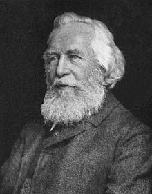
(Portrait of Ernst Haeckel, courtesy of Wikipedia.)
Phylogenetic trees are a framework in which one studies how species change with time, one of the goals being to try to understand which species are closer to one another than to other species. This suggests the idea of defining a distance between two species which would obey the nice properties that distances developed in mathematics for other reasons (Euclidean distance, taxicab distance, Hamming distance, etc.) might obey. Typically the distance between two objects P and Q (whether they are points, trees, or languages), d(P,Q), would obey the rules:
a. d(P,Q) is a non-negative real number.
b. d(P,Q) = d(Q,P)
c. d(P,Q) = 0 if and only if P = Q
d. For any three objects P, Q, R
d(P,Q) + d(Q,R) ≥ d(P, R)
(which is known as the triangle inequality).
So given two trees, how might we determine how far apart they are? Or put slightly differently, how can we measure similarity versus dissimilarity for trees, perhaps in some other way than using a "distance"? So if one thinks mathematically one might want to know what kinds of trees are allowed in the comparisons because trees come in many "flavors." A tree is a special kind of geometric diagram known as a graph, which consists of dots called vertices and line segments called edges. What makes trees special is that they have no "circuits" (sometimes called cycles) and consist of one piece. The fact that a tree is in one piece (the technical term is connected) means that one can move between any pair of distinct vertices along edges. A circuit is a collection of edges such that if one starts at a vertex one can walk back to the start using distinct edges. In Figure 5 we see a graph which has several pieces; it is not connected. The piece labeled H has 6 vertices and 7 edges and is not a tree--it has three different circuits. The other three pieces, considered together as a graph G in Figure 5, is called a forest, because each piece is a tree. Graph G (without part H) is not connected and consists of three separate trees. The unlabeled piece is a special kind of tree sometimes called a star. This star tree has 6 vertices and 5 edges.

Figure 5 (A graph which consists of 4 pieces, three of which are trees.)
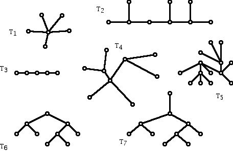
Figure 6 shows examples of 7 different trees that are all different from each other, that is, they are not isomorphic. In discussions of phylogenetic trees, typically there are some restrictions on the types of trees that are being looked at.
Figure 6 (Seven non-isomorphic trees.)
We will be particularly interested in trees where all of the vertices are either 1-valent or 3-valent (1 edge or 3 edges at a vertex), which are labeled or unlabeled, as well as the related graphs which are known as rooted binary trees, which have exactly one 2-valent vertex. One does have to be careful because not all scholarly work in this area uses the same definitions of terms that others scholars use. In particular, here I will disregard the issue of having direction on the edges (an arrow on one or more edges). In many discussions of phylogenetic trees the edges have a direction. In cases where trees are being used to show ancestral information, vertices towards the top are typically representing "older" things. Often in graph theory one concentrates on the number of edges and vertices of a graph in problem descriptions, but here we will be interested in the number of leaves (1-valent vertices) of a tree. One usually identifies the 1-valent vertices with the taxa (or language families) whose ancestry one is studying. For example, Figure 7 displays the two different (non-isomorphic) trees with 4 leaves.
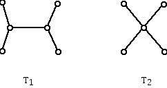
Figure 7 (Non-isomorphic trees with 4 leaves (1-valent vertices).)
But for what follows, we will not look at trees where there are valences (degrees) higher than three. From this point of view there is only one "topological type" of tree with 4 leaves and with the other two vertices having valence 3. Note that for the tree on the left, pairs of 1-valent vertices are not all alike. For example, the two 1-valent vertices on the left can be joined by a path of length two while the two 1-valent vertices at the top need a path of length 3 to join them.
There are many ways that mathematicians have expanded their study of trees from the first efforts of mathematicians like Arthur Cayley (1821-1895), who in part was interested in using trees as a model for chemical molecules, a practice that continues today. Graph theory finds many applications in chemistry. Before returning to the thread of ancestry ideas in genetics, let us "review" some more aspects of trees.
a. What are the degrees (valences) of the vertices of the tree?
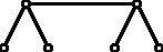
Figure 8 (A 4-leaf tree with two 3-valent vertices.)
Comment:
In the above tree diagram there are 6 vertices, and 5 edges. In general, trees have the property that there is always one more vertex than there are edges.
b. Does the tree have a special vertex called the "root?"
Comment 1:
In Figure 9 below there are two trees which are isomorphic (same structure) but have a rather different visual appearance because of the way they are drawn on the page. Both of these trees arise from the tree in Figure 8 by subdividing the horizontal edge of Figure 8. This subdivision process can be thought of as removing the edge and replacing it with a path of length 2, which has a 2-valent vertex in the path. This new vertex of degree 2 can be thought of as the "root" of the tree. From this perspective, for the tree in Figure 8 four of the edges give rise to rooted trees that are the "same" while when the horizontal edge is subdivided one gets a "different" rooted tree.
The tree on the left in Figure 9 is sometimes the style with which trees that are used for showing the "forks" in making a decision from a starting "root" are displayed. The tree on the right is often the style used for showing family trees and/or trees that show common ancestors of species or genes.
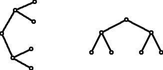
Figure 9 (Isomorphic rooted trees with four leaves.)
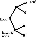

Figure 10 (Parts of the trees in Figure 9 identified.)
Comment 2:
The concept of the root of a tree may be familiar if you have looked at genealogical trees drawn to look at one's family ancestors. Your genealogical tree may show your "great maternal grandmother" Eve as its root and have labels that show how Eve married and who her children were and who the spouses and children of her children were. Some families are complicated when an ancestor has children by one partner and then marries again and has other children. Other terminology for trees in biology makes reference to the 1-valent vertices as leaves and the non-leaf vertices other than the root as the internal vertices of the tree.
Comment 3:
Both of the non-leaves of the tree in Figure 8 are of valence 3. When one picks an edge of such a tree to place a root on, this can be done by using any edge of the tree. However, sometimes the resulting rooted trees, arising from different edges which can be subdivided to create a root, can be isomorphic. Figure 11 shows how to subdivide an edge in Figure 8 to get a tree that can be thought of as rooted using the 2-valent vertex at the top so that the resulting tree is not isomorphic to the trees in Figure 10. One way to see this is that Figure 11 has a leaf that is joined to a 2-valent vertex while the graph in Figure 10 has no leaf of this kind.

Figure 11 (Rooted tree not isomorphic to the ones in Figure 10..)
c. Are you interested in comparing the distance between any pair of vertices in a tree or only vertices which have particular properties? For example, sometimes one is interested in the distance between the leaves of a tree or between the root of a tree and its leaves, or between the "internal" vertices of a tree--vertices of an unrooted tree which are not leaves.
d. Are there labels assigned to the vertices and/or edges of the tree?
Comment:
Sometimes in a diagram vertices/edges are labeled as a convenience to be able to "talk about" which vertex or edge one has in mind when referring to a vertex or an edge. However, sometimes the labels are part of the mathematical model (representation) that the graph is being used to construct. For example, in Figure 12 we have some graphs (trees in fact) with the labels homo sapiens (H), baboon (B), gorilla (G). Do you think all three drawings with their labels are different, or do you think that the top two drawings are "isomorphic" (have the same structure)?
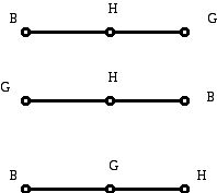
Figure 12 (Trees with vertex labels.)
e. Are there weights located at the vertices of the tree?
Comment:
One might want to have a labeled rooted binary tree where the root vertex is assigned the weight 0, which represents the time in the past when a "clock" was started. Now the weights at other vertices are the time when an event occurred as indicated by the presence of that vertex. Sometimes only the root is labeled (0) and the leaves.
f. Are their weights indicated for the edges of the tree?
Comment:
Weights on edges might indicate some way of saying how far apart the ends of the edges are. In Figure 12 we might put weights on the edges in the tree at the top to indicate whether gorillas were closer to humans or baboons were closer to humans. For this kind of model one has to decide if summing edges along a path is meaningful or not.
Comments?
Phylogenetic trees
Now suppose we want to label the leaves of our trees (rooted or unrooted binary trees with taxa (species)), and we want to see how many different ways there are to do this. Consider the example of such a tree with four leaves. The number of ways to choose labels for the two 1-valent vertices of the tree T1 on the left in Figure 7 is 4C2. This quantity counts the number of ways to select combinations of two things from 4, where order does not matter. If you are not familiar with how to calculate this number, which is 6, you can just count them all: A, B; A, C; A, D; B, C; B, D; and C, D, where we are using the letters A, B, C and D as the 4 labels. Note that the order of the selection does not matter, the selection of B and C is the same as the selection C and B. Figure 13 shows the three ways of labeling the tree on the left of Figure 7 with labels drawn from the four labels A, B, C, and D.
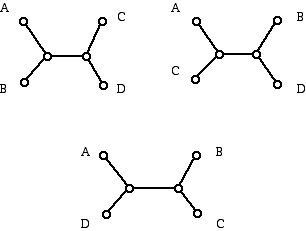
Figure 13 (The three different ways to label the one binary tree with 4 leaves with 4 labels on the leaves.)
Why don't we show three additional trees with the other pairs of labels for the vertices which are 1-valent to the left? The answer is that when we select a pair, say B and C, we have also selected the pair A and D. Thus, the 3 labeled trees in Figure 13 already show the different ways that a pair of labels can appear at 1-valent vertices that are two units apart (connected with a path of length 2) or at 1-valent vertices that are three units apart (connected with a path of length 3). What we have done here is a very common thing in mathematics. When it suits our purpose to think of two things that look different to be the same we do it! It is similar to the fact that the fractions 2/4 and 3/6 look different from 1/2 and each other, but we still think of these three fractions as representing the same number.
Note that for the tree on the right in Figure 7 if we label the leaves for this tree with a distinct letter from A, B, C, D (thus, all 4 leaves have different labels) there is a sense in which one might say all the different ways of labeling the tree on the right are equivalent. However, for the tree on the left in Figure 7 it is natural to think of the 3 trees shown in Figure 13 as being different.
You may be wondering for a tree whose vertices are 1-valent and 3-valent how many different (non-isomorphic) labeled trees there are with n leaves.
Fact:
If a tree has 1-valent and 3-valent vertices and only its leaves are to be labeled where the number of leaves is n (n being 3 or more), then:
i. The tree has n-2 internal vertices
ii. The tree has n-3 internal edges
iii. There are 1(3)(5)....(2n -5) different such labeled trees.
Note that if b(n) (binary trees) denotes the number of trees we are counting, then
b(n ) = b(n -1)x(2n -5) = 1(3)(5)...(2n -5) (*)
If there are n leaves, the number of edges in our tree is n (leaf edges) + (n -3) internal edges for a total of 2n -3 edges. For a tree with n-1 leaves we have (n -1) leaf edges together with n-4 internal edges or 2n -5 edges total. In our count in going from trees with n-1 leaves to a tree with one more leaf, for each "old" tree we can get (2n -5) new ones, since we can add a new 3-valent vertex (by subdividing an edge and attaching a 1-valent vertex) on any existing edge. We can try checking equation (*) above for n = 4. We get (since 2 x 4 - 5 = 3) 1 x 3 = 3 which is the number of trees we got in Figure 13. For n equal to 5 we get 15 trees. The size of b(n), the number of binary labeled trees grows very rapidly, meaning that the computational work for solving many phylogenetic problems seems not to be doable with algorithms that work in polynomial time.
What about rooted labeled trees? For each labeled tree with n leaves there are n leaf nodes and n-3 internal edges for a total of 2n -3 edges. The root we select can be placed on any of these edges, so to find the number of labeled rooted trees with n leaves we need to multiply equation (*) by (2n -3) obtaining
rooted b(n) = 1(3)(5)...(2n -5)((2n -3) (**)
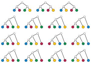
Thus, for n = 4 we should have 15 such trees with 4 leaves. Can you find them all? (Check your answer against Figure 14 where the labels are colors rather than letters.)
Figure 14 (15 rooted binary trees with 4 leaves labeled, courtesy of Wikipedia.)
It is worth noting that we are considering two labeled trees the same if the order of the two labeled leaves below a vertex of degree 3 are switched . Thus, for the first row of the leftmost tree in Figure 14, had the blue and red labels been switched, we would consider this the "same" tree. The trees in the top row of Figure 14 are those that arise from rooting the one fully internal edge of the trees in Figure 13.
Many people find diagrams such as those in Figures 7 and 13 an entry point into getting insights into trees and labeled trees. Others want something more algebraic, and typically computers can't be used to help with calculations when they have to work on diagrams rather than strings of symbols. So for those who like to think about things in a more "algebraic" way, one can get equations which show relations expressed by the geometry in the pictures of graphs. Since a tree with n vertices has n-1 edges, and every tree (other than the trivial tree, the tree consisting of a single vertex) has at least two 1-valent vertices), we can try to count the number of 1-valent vertices of a tree in terms of the other degrees of vertices in the tree. If a tree has ti vertices of valence i (degree i) we can derive the equation below. The key idea is that adding up the degrees of the vertices counts each edge twice, once at each end (together with the fact that there is one more vertex than there are edges in a tree).
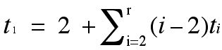
Note that for counting the number of 1-valent vertices in a tree the number of 2-valent vertices does not play a role. Of course, one needs to count the number of 2-valent vertices to see what the total number of vertices in a tree is. You can check that since the bottom tree in Figure 13 has two vertices of degree three, it has four 1-valent vertices.
There is also the theory of splits, which we will look at for trees with vertices of degree 1 and 3 (such as those in Figure 13) where the leaves have distinct labels. However, the idea carries over to labeled trees in general. Since each edge when cut with a scissors divides the tree into two pieces we can for each edge record the labels in the two pieces into which the tree is cut. I will use the notation U | V for the "split" of the labels into two sets, where the split U | V is the same as the split V | U.
Here are the splits for the lower tree in Figure 13:
{A} | {B, C, D}
{B} | {A, C, D}
{C} | {A, B, D}
{D} | {A, B, C}
{A, D} | (B, C}
Of the 5 splits above, each of the other two trees in Figure 13 would have these splits as well but the last split above "codes" the fact that the bottom tree is "different" as a labeled tree from the two above it (up to permutations of the labels).
The "essential" splits (those for edges that connected two non-leaf vertices) for the other two trees are:
Left tree:
{A, B} | {C, D}
Right tree:
{A, C} | {B, D}
Thus, we can tell trees apart using their splits instead of relying on visual aspects of trees to cue us that they are different.
The notion of splits can also be used to construct a distance between two trees, in what is known as the Foulds-Robinson distance (L.R. Foulds and D. F. Robinson) between two trees. (Usually, author names for scholarly papers in mathematics are listed in alphabetical order but for the paper that introduced this distance, Robinson's name is listed first.)
Given two sets A and B one can compute the symmetric difference between the two sets, which consists of those elements which are in A or B but not both. So the Robinson-Foulds distance between two trees (it can be done for more general trees and splits than the binary unrooted tree case we looked at above) builds on the notion of symmetric difference of sets. Suppose we are given trees T and T*. If S(T) is the number of splits of tree T which are not present for T* and S(T*) is the number of splits of T* which are not present for T, then d(T,T*) = S(T) + S(T*). This distance is relatively easy to compute for sizable trees but it tends to reflect small changes in tree topology in a way which is not "ideal." Also the behavior of this distance on random trees is not ideal. However, the attempt to use this distance in phylogenetic problems has been responsible for research about the properties of this distance function for trees which is of interest for "theoretical" reasons. Also, to the extent that its properties are not "what one wants" it encourages other researchers to find better ideas for finding the distance between trees.
Graphs are a wonderful tool for studying many parts of mathematics. All of you are probably familiar with examples of convex polyhedra such as the tetrahedron and the cube. For example, here is a diagram of the tetrahedron drawn as a graph in the plane.
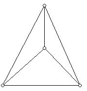
Figure 15 (Graph of the tetrahedron drawn in the plane.)
It turns out that all polyhedra with all of their vertices of degree three can be generated from the tetrahedron by a sequence of "graph transformations." This fact is a special case of what is known as Steinitz's Theorem. Here is a diagram that shows the way to make such a transformation. One picks two edges that bound the same region (called a face) and join them as shown in Figure 15 which is a schematic. The only face that is shown is the one where two edges have been chosen and this face is "split."
Figure 16 (A face split for generating 3-valent convex polyhedra from the tetrahedron.)
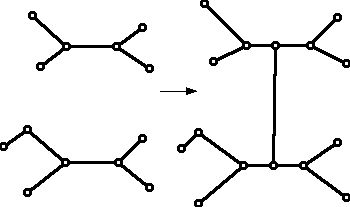
There are many theorems about how to "modify" graphs which already have a property (say that they represent the edge-vertex graph of a convex polyhedron) and show how to get a new and different graph with the same property. The theory of phylogenetic trees also involves taking trees and showing how to change them or piece them together to get a "related" tree that has the properties one wants. For example Figure 17 shows how to take two trees on the left, where each of these trees has vertices of degree 1 and 3, and perhaps at most one vertex of degree 2, and piece them together to form a new tree with the property that it has vertices of valence 1 and 3 and at most one vertex of valence 2. The process is done in such a way that the number of 1-valent vertices is the sum of the sum of 1-valent vertices in the separate trees.
Figure 17 (A method for piecing together a bigger tree from two smaller trees.)
If the first tree was built from one set of species and the second from a disjoint set of species, one might try to piece together the two trees to get a tree based on the larger collection of species in some way.
To tell how far apart two species are one can conceive of various different approaches, each of which might give different insights.
a. If one had the whole of the human genome from start to finish and the chimp genome from start to finish, one could compute the "distance" between the two genomes.
b. If one had a list of corresponding genes for humans and for chimps one could for each gene compute the distance between these genes. One could then measure how far apart the two species were by summing the distances between the genes.
In the world of phylogenetic trees one can use similar distinctions in order to build a tree which shows the "ancestry" relations between a collection of species of interest, say the primates, the birds, or a collection of viruses. However, as noted above, the tree one constructs might merely be one which shows the connection relationships or might try to do more and indicate "distance" relationships for the primates.
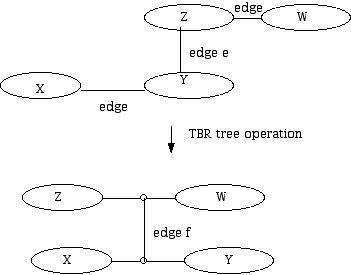
Many "operations" or transformations of one tree to another tree have been conceived of and discussed in view of species closeness issues and mathematical motivations. One wants to see the minimal number of steps to transform one tree to another with the same number of leaves, as some measure of "distance." Three particular operations are well studied. In the sequence of diagrams below, these three operations known as TBR (tree bisection and reconstruction), SPR (subtree prune and regraft) and NNI (nearest neighbor interchange) are explored by the use of diagrams. If a transformation results in a 2-valent vertex such vertices are "suppressed" in these transformations, so that the only trees obtained are ones which have 1-valent and 3-valent vertices. However, sometimes more general versions of trees are used with operations of this spirit.
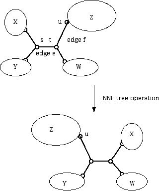
Figure 18 (The NNI operation on a tree.)
Note that in Figure 18 the elements in the sub-pieces of the tree consisting of blobs Z and Y are closer after the switch than before. Here, we switched the blobs X and Z but you might think about switching the blobs X and W instead.
Figure 19 (TBR tree operation.)
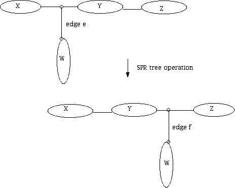
Figure 20 (SPR tree operation.)
Again, the tree one constructs could be based on how far apart pairs of species are in terms of their whole genomes or one could construct a family of trees which is constructed on the basis of using each gene that can be compared across the species to find a tree associated with that gene. Now one has a collection of trees, each one based on a different gene and one can try to construct a single tree which is the most "consistent" with the given collection of trees that would represent the species as a whole. Various ways can be devised for constructing such a "consensus" tree but typically the different methods yield different trees. The insights have been helped by the mathematics which attempts to understand how to choose a winner in an election where there is information about how members of a group vote.
In a rapidly emerging field like computational biology (computational genetics), mathematics has benefited as much as biology (genetics) from the attempts of the mathematically trained to use existing or new ideas to help get further comprehension. Over a period of time these ideas and insights become the foundations of whole new pieces of the mathematical and biological landscape. Many mathematicians and biologists continue to inspire each other in getting a better understanding of both the world of mathematics and the world of biology.
Comments?
References
Alon, N. and H. Naves, B. Sudakov, On the maximum quartet distance between phylogenetic trees, SIAM J. Discrete Math 30 (2016) 718-735.
Bryant, D. Building trees, hunting for trees and comparing trees, Doctoral Thesis, U. of Canterbury, 1997.
Clote, P. and R. Backofen, Computational Molecular Biology, Wiley, New York, 2000.
Felsenstein, J. Inferring Phylogenies, Sinaur, Sunderland, 2004.
Finden, C., Obtaining common pruned trees, J. of Classification 2 (1985) 255-276.
Gusfield, D., Algorithms on Strings, Trees, and Sequences, Cambridge U. Press, New York, 1997.
Gusfield, D., ReCombinatorics: The Algorithmics of Ancestral Recombination Graphs and Explicit Phylogenetic Networks, MIT Press, Cambridge, 2014.
Hall, B., Phylogenetic Trees Made Easy, Sinauer, Sunderland, 2004.
Hein, J. and M. Schierup, C. Wiuf, Gene Genealogies, Variation and Evolution, Oxford, New York, 2005.
Jansson, and C. Shen, W-K Sung, An optimal algorithm for building a majority rule consensus tree, RECOMB 2013, 2013, p. 88-99, Springer.
Jones, N. and P. Pevzner, An Introduction to Bioinformatics Algorithms, MIT Press, 2004.
Klein, P., Computing the edit-distance between unrooted ordered trees, in G. Bilardi et. al. (Eds.), ESA 98, LNCS 1461, pp. 91-102, 1990, Springer.
Lin, Y., and V. Rajan, B. Moret, A metric for phylogenetic trees based on matching, IEEE/ACM Transactions on Computational Biology and Bioinformatics, 9 (2012) 1014-1022.
Margush, T. and F. McMorris, Consensus-trees, Bull. Math. Bio. 43 (1981) 239-244.
Page, R. and E. Holmes, Molecular Evolution: A Phylogenetic Approach, Blackwell Science, Oxford, 1998.
Pevzner, P., Computational Molecular Biology, MIT Press, 2000.
Robinson, D., Comparison of labeled trees with valency 3, J. Comb. Theory 11 (1971) 105-119.
Robinson, D. and L. Foulds, Mathematical Biosciences 53 (1981) 131-147.
Semple, C. and M. Steel, Phylogenetics, Oxford U. Press, New York, 2003.
Strimmer, K. and A. von Haeseler, Quartet puzzling: A quartet maximum-likelihood method for reconstructing tree topologies, Mol. Biol. Evol., 137 (1996) 964-969.
Steel, M., Phylogeny, SIAM, Philadelphia, 2016.
Steel, M. and D. Penny, Distributions of tree comparison metrics--some new results, Syst. Bio., 42 (1993) 126-141.
Waterman, M., Introduction to Computational Biology, Chapman & Hall, London, 1995.
Those who can access JSTOR can find some of the papers mentioned above there. For those with access, the American Mathematical Society's MathSciNet can be used to get additional bibliographic information and reviews of some these materials. Some of the items above can be found via the ACM Portal, which also provides bibliographic services.
Joseph Malkevitch
York College (CUNY)
Email Joseph Malkevitch