Neural Nets and How They Learn

This column introduces neural nets, a programming paradigm designed to model biological neural tissue, and the mathematical theory that allows them to learn to improve their performance. ...

Introduction

Computers are a lot better than me at some tasks. I wouldn't want to race a computer to find $\arctan(1.374)$, and if I need to find the most relevant web pages dealing with "linear algebra," I'll ask Google to do it for me.

But, in defense of my own processing unit, I'm pretty good at other things, such as reading my students' handwriting. For instance, I easily recognize these images as representing the digits 0 - 9.

In fact, I can even recognize with no trouble 2's or 4's drawn with different topological properties.

Of course, I wasn't born with this ability; I learned it over time by looking at a large number of examples.

By contrast, we think of computers as performing tasks that require them to process data using a finite set of rules that are known ahead of time. This doesn't seem to provide the flexibility they need to learn, to change their behavior based on experience in an effort to improve their future performance.

Machine learning, however, provides techniques that allow a program to learn from its experience. This column introduces neural nets, a programming paradigm designed to model biological neural tissue, and the mathematical theory that allows them to learn to improve their performance.

A brief explanation of neural tissue

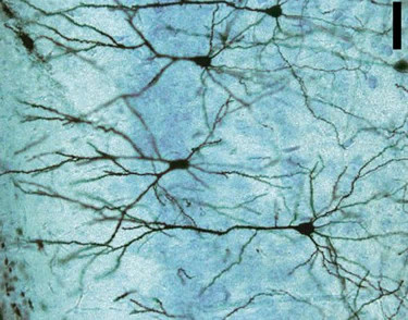
Shown here is a schematic drawing of a neuron, a specialized cell such as one in the human nervous system. In extremely simplified terms, a neuron utilizes an electro-chemical process to evaluate input information and make decisions.

A neuron takes in information through dendrites, the spindly tentacles on the left that we may think of as input channels. In its resting state, the neuron maintains a concentration of ions inside the neuron that creates an electric potential of -70 mV across the cellular membrane. Signals received through the dendrites can affect this potential by changing the concentration of these ions inside the neuron. If the electric potential is increased beyond some threshold value, the neuron is activated and responds by raising the electric potential to 40 mV. This creates a strong electrical signal, known as the action potential, that is transmitted along the axon, which is shown on the right above and which serves as an output channel.

Neurons are chained together through a system of synapses, junctions in which an axon (output) of one neuron is joined to a dendrite (input) of another. Synapses exhibit different types of behavior by modulating the action potential conveyed from one neuron to the next. First, the strength of the signal carried by the action potential varies from one synapse to another. Second, a signal received by a neuron through one synapse may cause the electric potential to increase, which makes it more likely that the neuron is activated. Such a synapse is called excitatory. Conversely, a signal received through another synapse may lower the electric potential, thus making it less likely that the neuron is activated. We call these synapses inhibitory.

To recapitulate, we will call attention to two important parts of this process. First, each neuron has a threshold that its electric potential must reach before activation. Second, each synapse conveys the action potential from one neuron to another with varying strength and effect.

What is most remarkable is that a neuron's activation threshold and the synapses' conveyance properties can change, and in this way, neural tissue is able to reorganize itself to improve its performance. This is what it means for neural tissue to learn.

A mathematical model of neural tissue

We will now create a simple mathematical model of a neuron, which will turn out to form the building blocks of our neural nets. Let's begin with a simple model of a neuron.

Suppose that we want to predict whether an Olympic athlete will win a medal in the half-pipe. There are many factors we may use in making our prediction, but we will keep it simple by focusing on three:

• $x_1$ is the number of hours that the athlete has trained before the event,
• $x_2$ is the number of chocolate donuts the athlete eats in the hour before the competition, and
• $x_3$ is the number of times the athlete has streamed Taylor Swift's latest album.

 

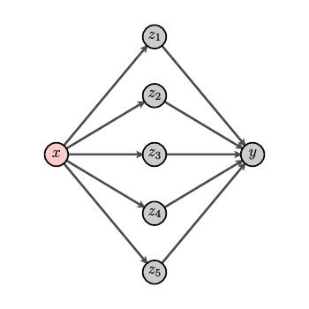
Here is a model of our neuron. The inputs $x_1$, $x_2$, and $x_3$ are carried to the neuron through synapses where they are processed into the output $y$.

 

Remembering that the synapses exhibit either excitatory or inhibitive behavior of varying strengths, we assign a weight $w_i$ to each synapse and aggregate the inputs as $$ w_1x_1 + w_2x_2 + w_3x_3. $$ An excitatory synapse will have a positive weight while a inhibitive synapse will have a negative weight.

Remember also that the neuron is activated when the aggregated signal from the dendrites reaches some threshold $\theta$. We then define $$ y = \begin{cases} 1 & \text{if } \sum_i w_ix_i \geq \theta \\ 0 & \text{if } \sum_i w_ix_i \lt \theta. \\ \end{cases} $$

If we want to use this model to make predictions, we need to choose values for the weights $w_i$ and the threshold $\theta$. We could begin using our intuition. It seems like $x_1$, the number of training hours, should make a significant excitatory contribution to the athlete's performance. Therefore, we might choose $w_1$ to a large positive number. It's probably not a good idea to eat a lot of chocolate donuts before a competition so we expect $x_2$ to play a strongly inhibitive role. We could assign a negative number with a fairly large magnitude to $w_2$. And while the haters may want to choose $w_3$ to play a similarly inhibitive role, we would realistically choose $w_3$ to be close to zero, which means that listening to Ms. Swift probably doesn't affect the athletes' performance significantly.

Of course, when we choose the weights $w_i$ and threshold in this way, we are really just guessing. Is there a way that we can get our neuron to learn? We know that neural tissue is able to adjust the weights and thresholds in response to experience and in an attempt to improve its performance. Suppose we have some data about athletes that assesses their performance and records the values of the inputs $x_1$, $x_2$, and $x_3$. Can we find a way to use this data to make optimal choices for the weights and threshold? This would be a mathematical approach to modeling the learning process.

We will explore this question a little later after we first put these ideas into a more general framework.

Comments?

Neural nets

Roughly speaking, there are three types of biological neurons: sensory, processing, and motor neurons. Sensory neurons are activated by changes in our environment and motor neurons activate a muscle or gland. These serve as inputs and outputs for the tissue. The processing neurons determine an appropriate response to the information relayed by the sensory neurons and send that response to the motor neurons.

To push our mathematical model of neural tissue a bit further, we will imagine connecting neurons to one another as shown here.

 

The neurons are arranged in layers beginning with an input layer on the left. Neurons in the input layer are connected to neurons in the first hidden layer and so forth. We call this structure a neural net.

Let's imagine how this might look in practice by considering how we might form a neural net to recognize handwritten digits. Our goal would be to input an image, such as one of the ones below, to the neural net and output the correct digit.

 

The digits shown here are from a publicly available source of digits called the MNIST database, which was originally created by the National Institute of Standards and Technology. This database contains 70,000 images; each image is a $28\times28$ array of pixels, and each pixel records a grayscale between 0 and 255.

These 70,000 images are broken into a group of 60,000 "training images" and 10,000 "test images." As will be seen shortly, we use the training images to choose the weights of each synapse and the threshold of each neuron to optimize the accuracy with which our net identifies digits. We then use the testing data to confirm that our choices generalize to a new set of data.

When we input the image into the neural net, we will feed in the grayscale value of each pixel. This means that there are $28^2 = 784$ inputs, $x_1, x_2, \ldots, x_{784}$.

Our net will have 10 outputs, $y_0, y_1, \ldots, y_9$. When we input an image that represents the digit $k$, we would like $$ y_j = \begin{cases} 1 & \text{if } j = k \\ 0 & \text{if } j \neq k. \\ \end{cases} $$

We now have a good sense of what the input and output layers look like. Adding layers between them, so-called hidden layers, gives our net more resolving power to identify digits. Suppose, for example, that there are no hidden layers so that the input layer is connected directly to the output layer. This means that each output, say $y_0$, is determined by our choice of 784 weights and one threshold. We could likely improve our net's ability to identify a "0" if we have more parameters to choose. Adding hidden layers gives us those parameters.

We will now introduce two relatively small changes to our model of a neuron whose use will become clear shortly. First, we earlier said that the output of a neuron is 1 when the condition $$ \sum_i w_ix_i \geq \theta $$ is satisfied. As we will see, it is more convenient to introduce the bias $b=-\theta$ and write this condition as $$ \sum_i w_ix_i + b \geq 0. $$

Second, the output of one of our neurons is currently either 0 or 1. If we define $z=\sum_i w_ix_i+b$, then the output as a function of $z$ is a step function.

 

Because it will useful to allow a continuous range of outputs between 0 and 1, we introduce the sigmoid function $$ \sigma(z) = \frac{1}{1+e^{-z}}. $$ As the graph below shows, $\sigma(z)$ is a continuous approximation to the step function.

 

We now define a neuron's output to be $$ y = \sigma\left(\sum_i w_ix_i + b\right). $$ Our condition that $y=1$ if $\sum_i w_ix_i + b \geq 0$ is replaced by $y \geq 0.5$ if $\sum_i w_ix_i + b \geq 0$. We may therefore interpret the output function $y$ as the confidence we have in the result or the probability that our prediction is correct. For instance, in our attempt to identify handwritten digits from an image, we could interpret $y_7$ as the probability that the digit is a "7".

Universality

Before we investigate how a training data set can be used to improve the performance of a neural net, it's worth thinking about the power of these nets. Consider, for example, the problem of identifying handwritten digits. An input image's grayscale values form the components of a vector in ${\mathbb R}^{784}$. The outputs $y_k$ form a vector in ${\mathbb R}^{10}$. Our neural net may be seen as an attempt to approximate the identification function $i:{\mathbb R}^{784} \to {\mathbb R}^{10}$. Is it reasonable to expect that a neural net can approximate such a function accurately?

We will illustrate by considering the simpler situation where we have a continuous function $f:{\mathbb R}\to[0,1]$ with one input and one output. We will show how to create a neural net with one hidden layer that approximates $f$ to any desired degree of accuracy on a closed and bounded interval.

 

 

We will first focus on a neuron in the hidden layer. Given an input $x$, we will denote the output of the $i^{th}$ neuron in the hidden layer by $z_i$. With an appropriate choice of weight and threshold, the function $z_i(x)$ can approximate a step function where the step occurs at some location $x=s$.

 

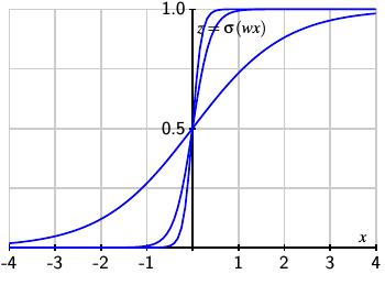
Let's consider a single neuron with weight $w$, an initial bias $b=0$, and output $z(x)=\sigma(wx)$. As we increase the weight $w$, the function $z(x)$ more closely approximates a step function. The figure below, which shows the results when $w=1$, $w=5$, and $w=10$, illustrates the improving approximations.

 

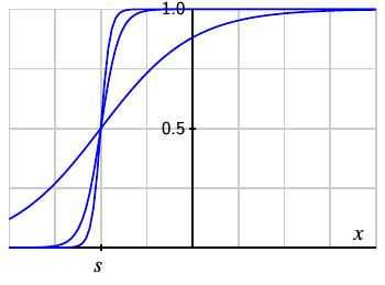
Furthermore, we can shift the location of the step by defining $z(x) = \sigma(w(x-s))$. As we increase $w$, we see that we form improving approximations to the shifted step function.

 

Therefore, with a large weight $w$ and a bias $b=-s/w$, the output of one neuron can be made to approximate a step function.

Let's now turn to the net's output $y$, which we want to approximate the function $f(x)$; that is, $$ y = \sigma\left(\sum_i w_iz_i(x) + b\right) \approx f(x). $$ In other words, we would like to find weights $w_i$ and bias $b$ such that $$ \sum_i w_iz_i(x) + b \approx (\sigma^{-1}\circ f)(x). $$

If we define $g = \sigma^{-1}\circ f$, we see that our task is to find weights $w_i$ and bias $b$ such that $$\sum_i w_iz_i(x) + b \approx g(x). $$

Suppose that our function $g(x)$ is as shown.
We will sample the function $g(x)$ at a finite number of points
and approximate $g$ by step functions that extrapolate between the values of $g$ at the sampled points.

We first choose the neurons in the hidden layer so that the function $z_i$ approximates a step function whose step occurs at the midpoint of the $i^{th}$ sampling interval.

For the single neuron in the output layer, we choose the bias $b$ to be the sampled value of $g$ at the left endpoint. We choose the weights $w_i$ to give the appropriate step over the $i^{th}$ interval so that $$ \begin{aligned} g(x) & \approx \sum_i w_iz_i + b, \\ \text{or } \hspace{12pt}f(x) & \approx \sigma\left( \sum_i w_iz_i + b\right).\\ \end{aligned} $$ By increasing the number of sampling points, we can in this way approximate the function $f$ to any desired accuracy over the closed and bounded interval.

More generally, given a continuous function $f:{\mathbb R}^n\to[0,1]^m$, we can find a neural net approximating $f$ to any desired accuracy on a compact subset. This is known as the universal approximation theorem for neural nets.

The significance of the theorem is illustrated by the problem of recognizing handwritten digits where the identification function is $i:{\mathbf R}^{784} \to [0,1]^{10}$. The approximation theorem says that there are neural nets approximating this function to any desired accuracy. We can therefore begin to search for such nets with the assurance that they exist.

The argument we gave for the universal approximation theorem says something else significant. To improve our approximations, we need to add more sampling points and therefore more neurons in the hidden layer. This points to the fact that we can improve the power of our nets by adding neurons into the hidden layers. The trade off, as we will see, is that larger nets require more effort to optimize.

Comments?

Modeling the learning process

As described earlier, neural tissue can reorganize itself, by adjusting the properties of its synapses and the activation thresholds of its neurons, to improve its performance. We would like to model this behavior in our neural nets. In particular, we would like to modify the weights and the biases in a net to optimize its performance.

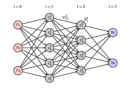
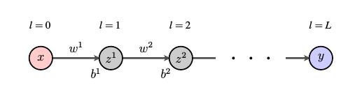
Let's introduce some notation before digging into this problem. Consider the following net, which has an input layer, an output layer, and some hidden layers.

The layers will be indexed by $l$ with $l=0$ describing the input layer and $l=L$ describing the output layer. Remember that the bias is a property of each neuron so $b^l_j$ will denote the bias of the $j^{th}$ neuron in layer $l$.

 

Each synapse has a corresponding weight so we denote by $w^l_{jk}$ the weight of the synapse connecting the $k^{th}$ neuron in layer $l-1$ with the $j^{th}$ neuron in layer $l$. We then have $$ z^l_j = \sigma\left(\sum_k w^l_{jk}z_k^{l-1} + b^l_j\right). $$

We think of this neural net as describing a function $f:{\mathbb R}^n\to{\mathbb R}^m$ where $n$ is the number of inputs and $m$ the number of outputs.

To make our goal more concrete, let's go back to the problem of identifying handwritten digits from an image of the digit. The identification function $i:{\mathbf R}^{784}\to{\mathbb R}^{10}$ has the property that, say, $i({\mathbf x}) = (0,0,1,0,0,0,0,0,0,0)$, if the image represented by $\mathbf x$ is a "2".

The task before us is to choose the weights $w^l_{jk}$ and the biases $b^l_j$ so that the function $f$ defined by the neural net effectively approximates the identification function $i$.

Remember that the MNIST database of handwritten digits includes 60,000 "training" images, ${\mathbf x}_1, {\mathbf x}_2, \ldots, {\mathbf x}_{60000}$. We will choose the weights and biases so that the differences between the neural net and the identification function is as small as possible on these training images. More specifically, we seek to minimize a least-squares function $E$ that measures the total difference in the net's output $f({\mathbf x})$ and the identification function $i({\mathbf x})$: $$ E = \frac 12 \sum_m \left|\left|f({\mathbf x}_m) - i({\mathbf x}_m)\right|\right|^2 $$ where the sum is taken over all the training images. The function $E$ is a function of the weights and the biases so that $$ E = E(w^l_{jk}, b^l_j), $$ and we want to find $w^l_{jk}$ and $b^l_j$ that minimize $E$.

This sounds like a classic optimization problem in calculus so our first idea may be to find the critical points of $E$ by solving the equations $$ \frac{\partial E}{\partial w^l_{jk}} = 0, \hspace{12pt} \frac{\partial E}{\partial b^l_{j}} = 0. $$ Unfortunately, this is not practical given the large number of weights and biases.

Instead, we choose an iterative approach known as gradient descent. Denoting the weights as $W=\{w^l_{jk}\}$ and biases as $B=\{b^l_j\}$, we first choose random values for the initial weights and biases $(W_0, B_0)$. Most likely, our choice does not minimize $E$, but, as we will describe shortly, we can compute the gradient $\nabla E(W_0,B_0)$, which tells us which direction to move in to decrease $E$. We take a small step in the direction opposite the gradient by defining $$ (W_1, B_1) = (W_0, B_0) - \epsilon \nabla E(W_0, B_0). $$ That is, our next set of weights and biases $(W_1, B_1)$ are obtained from our randomly chosen weights and biases $(W_0, B_0)$ by moving a little ways in the direction of $-\nabla E(W_0, B_0)$. This has the effect of decreasing the error so that our new neural net is a better approximation of the identification function $i$ on the training data.

In other words, the neural net has improved its performance on the training data. It has learned!

Of course, we can repeat this process: $$ \begin{aligned} (W_2, B_2) & = (W_1, B_1) - \epsilon \nabla E(W_1, B_1), \\ (W_3, B_3) & = (W_2, B_2) - \epsilon \nabla E(W_2, B_2), \end{aligned} $$ and so forth. At each step, we can expect the performance of the net to improve.

The parameter $\epsilon$ is called the "learning rate." With a large value of $\epsilon$, we take large steps and may possibly overshoot the minimum. With a small value of $\epsilon$, we take small steps and may require many steps to get near the minimum of $E$. Clearly, some thought needs to go into the choice of $\epsilon$.

Backpropagation

The outline of our gradient descent algorithm is now clear. What remains is to devise a way to compute the gradient $\nabla E$. Remember that there are likely thousands or even millions of weights and biases, and computing the gradient of a function with a million variables seems like a daunting task. Fortunately, there is an extremely efficient algorithm for computing $\nabla E$, which is known as backpropagation and which we will describe here. As it happens, this was also the topic of a recent Feature Column on automatic differentiation.

We will explain the backpropagation algorithm using a simple net in which each layer has only one neuron. This demonstrates the essential idea of backpropagation while simplifying the notation.

 

In this case, we need to compute the partials $\frac{\partial E}{\partial w^l}$ and $\frac{\partial E}{\partial b^l}$. In our notation, $f(x) = y(x)$ and since $E = \frac 12 \sum_m \left(f(x_m) - i(x_m)\right)^2$, we have $$ \frac{\partial E}{\partial w^l} = \sum_m \frac{\partial}{\partial w^l}[y(x_m)] \left(y(x_m) - i(x_m)\right). $$ We find a similar expression when we compute $\partial E/\partial b^l$, which means that we only need to compute the partials $$ \frac{\partial y}{\partial w^l} \text{ and } \frac{\partial y}{\partial b^l} $$ for each training datum $x$ in order to find the gradient $\nabla E$.

In a "forward" pass through the neural net, we begin with a piece of training data $x$ and, moving left to right, compute $$z^l = \sigma\left(w^lz^{l-1} + b^l\right) $$ for each $l$. This expression also applies if we set $y=z^L$ and $x=z^0$. For the time being, notice that the Chain Rule implies $$ \begin{aligned} \frac{\partial z^l}{\partial z^{l-1}} & = \sigma'\left(w^lz^{l-1} + b^l\right)w^l, \\ \frac{\partial z^l}{\partial w^{l}} & = \sigma'\left(w^lz^{l-1} + b^l\right)z^{l-1}, \\ \frac{\partial z^{l}}{\partial b^l} & = \sigma'\left(w^lz^{l-1} + b^l\right). \\ \end{aligned} $$

After our forward pass, we make a second pass from left to right. We begin by noting that $$ \frac{\partial y}{\partial z^L} = \ \frac{\partial z^L}{\partial z^L} = 1. $$ We work our way backward through the layers using the Chain Rule: $$ \frac{\partial y}{\partial z^{l-1}} = \frac{\partial y}{\partial z^{l}} \frac{\partial z^l}{\partial z^{l-1}} = \frac{\partial y}{\partial z^{l}} \sigma'\left(w^lz^{l-1} + b^l\right)w^l. $$

We then have $$ \begin{aligned} \frac{\partial y}{\partial w^{l}} & = \frac{\partial y}{\partial z^{l}} \frac{\partial z^l}{\partial w^{l}} = \frac{\partial y}{\partial z^{l}} \sigma'\left(w^lz^{l-1} + b^l\right)z^{l-1} \\ \frac{\partial y}{\partial b^{l}} & = \frac{\partial y}{\partial z^{l}} \frac{\partial z^l}{\partial b^{l}} = \frac{\partial y}{\partial z^{l}} \sigma'\left(w^lz^{l-1} + b^l\right). \\ \end{aligned} $$

This is the essence of the backpropagation algorithm. Of course, our explanation is simplified by the fact that each layer has only one neuron, but the same idea applies more generally in spite of the fact that the notation becomes more unwieldly.

This is a remarkable algorithm. It is possible to prove that the computational effort required to evaluate the gradient in this way is no more than four times the effort to evaluate the function $f(x)$ on the forward pass. This efficiency allows us to work with powerful neural nets having many neurons in many hidden layers.

Additional considerations

We have now seen how neural nets can learn by using a set of training data to find weights and biases that minimize an error function on the training data. There are many other issues that we haven't touched on, however.

Since the iterative gradient descent algorithm will most likely never find the exact minimum of the error, we need to develop a stopping condition for the gradient descent. Remember that we earlier said that the MNIST database contained a set of 60,000 images that we called the training data and another set of 10,000 images that we called the test data. After each step of the gradient descent algorithm, we evaluate the error of our neural net applied to the test data. We should expect that, as we improve the net's performance on the training data, the improvement should generalize to the test data as well.

What typically happens is that the error on the training set decreases toward zero, but the error on the test data stabilizes at some positive value, as shown below.

As we continue refining the weights and biases, we continue to squeeze error out of the training data without seeing any improvement on the test data. This is because the training data almost certainly contains noise that does not appear in the test data. In this case, continuing to improve the performance on the training data just bakes the noise into the net. This is called overfitting. One simple approach to avoiding it is to end the gradient descent algorithm when we no longer see an improvement in the net's performance on the test data. There are, however, more sophisticated ways of tackling this problem.

 

There are other choices for the error function that improve the efficiency of the gradient descent algorithm. As we saw above, the derivatives of the error function are expressed in terms of the derivative of the sigmoid function $\sigma'(z)$. Since $\sigma(x) = 1/(1+e^{-x})$, it follows that $$ \sigma'(x) = \sigma(1-\sigma). $$ Looking again at the graph of $\sigma$ shows why this might be problematic.

Remember that the weights are initially randomly chosen. This means that we might accidentally chose the weights to be far away from where they should optimally be. In particular, a neuron may get stuck evaluating to something close to, say, $\sigma = 0$ when it should optimally evaluate to $\sigma = 1$. Given the form of $\sigma'$, the derivative will be quite small in this case, and it will take the gradient descent algorithm a long time to change the weights appropriately. For this reason, different choices for the error function can be advantageously used.

 

Comments?

Summary

Neural nets form a rich subject into which we have merely dipped our toes. In this brief introduction, however, we can see that neural nets provide a powerful tool for teaching a computer to classify data.

When we looked at the universal approximation theorem, we saw that we can increase the power of our nets by adding more neurons into the hidden layers. Working with a large number of neurons in many hidden layers is known as deep learning. The overwhelming size of the nets presents new opportunities as well as new challenges; addressing these challenges is the subject of a considerable amount of current work.

Neural nets are being applied to an increasingly wide range of problems. As we have seen in this article, it is possible to design nets that recognize handwritten characters. In fact, it's fairly easy to construct a net having 30 neurons in one hidden layer using 74 lines of Python code that correctly identifies 95% of the images in the MNIST test data set (see Nielson's book cited in the references). More generally, applications of neural nets are found in image detection, medical diagnoses, and stock market predictions.

Of course, a net is only as good as the data that we use to train it. Any biases that appear in the training data will be built into the net and influence any decisions that the net makes.

Equally troubling, perhaps, is that it is difficult to know how a trained neural net really works. The gradient descent algorithm finds nearly optimal weights and biases without human intervention. This means that we lose the ability to describe with any certainty the role of any particular neuron in the net. In some sense, we are trusting the net to make decisions without knowing precisely how those decisions are being made. This is sure to raise ethical concerns as neural nets become increasingly ubiquitous in our society.

References

• A. C. C. Coolen. A Beginner’s Guide to the Mathematics of Neural Networks. In Concepts for Neural Networks. L.J. Landau, J.G. Taylor (eds). Perspectives in Neural Computing. Springer, London. 1988.

  This paper explains the biological origins of the mathematical theory of neural nets.

• G. Cybenko. Approximation by Superpositions of a Sigmoid Function. Math. Control Signals Systems, Vol. 2, 303-314. 1989.

• David E Rumelhart, Geoffrey E. Hinton, Ronald J. Williams. Learning representations by back-propagating errors. Nature, Vol. 323, 533-536. October 9, 1986.

• Michael Nielson. Neural networks and deep learning.

  This online book is a thorough guide to neural networks written at an introductory level. Nielson includes lots of Python code that allows readers to experiment with the ideas. In particular, he presents a 74-line program that creates a neural net to classify handwritten digits with an accuracy of 95%. The argument that I have presented here for the universal approximation theorem also follows Nielson.

• Yann LeCun, Corinna Cortes, Christopher J.C. Burges. The MNIST Database of handwritten digits.

Comments?