Pretty as a Picture (Part II)
Here I will discuss how the other kind of graphs, those involving diagrams with dots and lines (see Figure 1) are also valuable in helping mathematical progress and in obtaining mathematical insights...
 Joseph Malkevitch
York College (CUNY)
Email Joseph Malkevitch
Images and physical models have spoken loudly to mathematicians over the years. Putting our visual system to work often suggests new patterns and new ideas that merely text based discussions of ideas fail to do. In a prior column I considered how mathematics has benefited by the discovery of the tools of analytical geometry so that pictures of algebraic equations called graphs could be drawn, making it possible for a dramatic interplay of algebra and geometry.
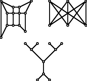
Here I will discuss how the other kind of graphs, those involving diagrams with dots and lines (see Figure 1) are also valuable in helping mathematical progress and in obtaining mathematical insights.
Figure 1 (Three different graphs, each of which consists of a single connected piece.)
Graphs (dots and lines variety)
Graphs of algebraic equations are familiar to American high school graduates because they are deeply embedded in the K-12 mathematics curriculum. However, dots and lines graphs are definitely not a part of the standard American K-12 public school curriculum though I think they should be. Graph theory belongs to the branch of mathematics known as discrete mathematics, while the other kind of graph also helps support the learning of continuous mathematics, the mathematics that leads to calculus, and beyond calculus to real and complex analysis.
While "graph theory" (see Figure 1) can be done without using diagrams--one can think of the vertices as nothing more than a set (collection of things), and the edges as a set of pairs of vertices--there is little doubt that many of these graph diagrams speak to those without mathematical training, just as they speak to geometers, combinatorists, and mathematicians whose expertise is with the "other kind" of graph.
Leonhard Euler (1707-1783) is generally given credit for the "discovery" of how to use graphs to get insights into mathematical questions, though the history of the use of "graph diagrams" for graph theory is complex. The credit given to Euler stems from his work on a problem in recreational mathematics known as the Koenigsberg Bridge Problem.
For those not already familiar with dots and lines graph theory, let me try to show the appeal of graph theory in a different way, one that indicates its usefulness in the world. It turns out that graph theory is a wonderful tool for people interested in mathematical modeling as an educational subject--using mathematics to get insights into problems that come up in daily life or on one's job. They are also a tool useful to those who use mathematics professionally, as well as those who might but typically do not. Thus, to solve a problem about efficient removal of snow from roads, one might want to find the route with the fewest repeated edges in the graph below, where each segment is assumed to have the same traversal time by a plow. More realistic versions of snow removal problems can also be solved with graph theory ideas. The graph shown in Figure 2 is known as a grid graph and represents the layout of sections of many villages, suburbs, and cities in America.
The plow is located at the dot in the upper left hand corner L. Can you see why there is no route for the plow that visits each of the street sections once and only once?
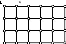
Figure 2 (A 3x5 grid graph which has 24 vertices.)
Before answering this question let us introduce some of the basic terminology of graph theory. Each dot in a graph diagram (Figures 1 or 2) is called a vertex, and several dots constitute a collection of vertices. The line segments (which could be curved or straight) that connect the vertices are called edges. The number of edges that meet at a vertex is called the valence or degree of the vertex. Thus, vertex L has valence 2 in Figure 2 while vertex vis 3-valent. The graph in Figure 2 has only 2-valent, 3-valent, and 4-valent vertices. It is a visually appealing image, symmetrical and "regular," and grid graphs model many situations that come up in urban life. Some graphs can be thought of as consisting of several pieces or components. Figure 1 can be thought of as having three separate pieces or each piece can be thought of as a single graph. A simple circuit in a graph is a tour using edges that starts and ends at the same vertex but "repeats" no other vertex and which uses distinct edges. I will refer to the tour in graph G as an Euler circuit (some call them Eulerian circuits).
Having introduced some graph theory terminology we can return to trying to connect up visually interesting examples with the role that these examples play in moving forward the progress of mathematics into understanding theoretical and applied problems. Why is it not possible to find a tour of the edges in Figure 2 for a snow plow that starts and ends at L that visits each edge once and only once for a connected graph? When a graph is not connected (a graph is connected if one can get between any two distinct vertices of the graph moving along edges of the graph), clearly the snow plow cannot get to all of the edges wherever it starts its tour from. Consider a vertex v that is not the initial vertex of the tour. Since one must enter v and leave on a different edge, because we are seeking a tour where edges are not repeated, we realize that any successful tour must use up edges in pairs--one to enter the vertex and one to leave it. Since the sum of even numbers is even, and since there are an odd number of edges at v, we see that no tour of the kind we desire is possible for this graph! What about the valence of the start vertex L? It, too, must have "even" valence (an even number of edges at a vertex), because if it is odd-valent we would leave L one more time than we could reenter it with an edge not already used. (Think about under what condition a graph might have a tour that visits each edge once and only once but starts and ends at different vertices.) Thus, if a graph has a single vertex which is "odd-valent" (a valence which is an odd number) it can't have an Euler circuit. When the vertices of a connected graph are all even-valent, it turns out that it is always possible to find an Euler circuit. Perhaps trying to find an Euler circuit for the very pretty graph in Figure 3 which is not only even-valent, but all its vertices have valence 4, will help you to see how to prove part (b) of the theorem below.

Figure 3 (A drawing of the graph of a 4-dimensional cube. All of the vertices of this graph are 4-valnet. Image courtesy of Wikipedia.)
Theorem (rooted in Euler's work):
a. If a connected graph has an Euler circuit then all of its vertices are even-valent.
b. If a connected graph has all of its vertices even-valent then the graph has an Euler circuit.
In the "center" of Figure 3 in the "thinner" style of edge representation you will see the graph of a 3-dimensional cube. Can you find other representations of 3-cubes in Figure 1? (Images suggest questions and ideas.) Do 3-dimensional cubes (where all of the vertices are 3-valent) have pretty drawings? You can look at Figure 4 to see which of these drawings of the 3-cube you find appealing and/or which suggest new mathematical ideas to you.

Figure 4 (Different ways to make a drawing of the graph of a 3-dimensional cube.)
When one thinks of the 3-dimensional cube, one thinks of a convex 3-dimensional solid with 6 vertices, 12 edges, and 8 faces all of which have 4 sides; in fact, the faces of a cube are squares. But the second row of the right-hand diagram in Figure 4 has regions that are not 4-gons. In light of this, why is this diagram a 3-cube? The issue is that there are places where edges cross/meet in Figure 4 that are not vertices of the graph involved. These "artificial" crossings arise as an artifact of the particular way that some of these graphs of the cube are drawn in the plane. The graph in the top row on the right and the middle row on the left are what are known as plane drawings of the cube. When one has a plane drawing of a graph the edges meet only at vertices. In the other diagrams drawn in the plane we can see edges that cross at points which are not vertices of the graph.
Planarity
Plane graphs are also referred to as graphs that have a planar embedding. Graphs that are "isomorphic" to plane graphs are called planar. Not all graphs are planar.
Figure 4 (top row) shows two versions of the graph of a 3-dimensional cube one of which has been drawn so that edges meet only at vertices (plane graph) and the other where edges do meet at points which are not vertices, but the two graphs are "structurally" the same — including the fact that they both have 8 vertices and 12 edges. While both graphs seem to divide up the plane regions, only plane drawings of graphs have regions that can be "defined" in a consistent manner and deserve the name faces. The 3-dimensional cube, after all, has 6 faces, each of the faces being 4-sided. The plane drawing shows these 6 faces with 4-sides but one has to get used to the fact that there is one region not like the others, called the "unbounded" or "infinite" face of the graph, though as you "walk around" its edges you get 4 sides. The reason why the drawing on the top left in Figure 4 is so common is that it is a drawing in the plane which suggests the 3-dimensionality of the cube. It is hard to see this aspect of the graph 3-cube from the other images in Figure 4.
So to begin with, do you find the drawings below (Figures 5 and 6) pleasing? They both arise in interesting ways in graph theory problems of interest or importance.

Figure 5 (The complete graph involving 5 vertices. It is often denoted K
5.)

Figure 6 (The complete bipartite graph involving two groups of 3 vertices. All the vertices in one group of vertices are joined to all the vertices in the other group, and there are no edges between the vertices in each group by itself.)
The famous theorem of Kazimierz Kuratowski (1896-1980) states that any graph which can't be drawn in the plane in essence has a "copy" within it of one of the two graphs above. The graph in Figure 5 is known as the complete graph on 5 vertices (often denoted K5) because there are five vertices each of which is joined to every other vertex with exactly one edge. The graph has 10 edges. (Can you find a formula for the number of edges of the complete graph with n vertices?) The graph in Figure 6 is known as the complete bipartite graph with exactly 3 vertices in each half of the bipartition, i.e. the two sets involved which are color coded here by red and blue. Each vertex of one color is joined to all of the other vertices of the other color and there are no other vertices. This graph has exactly 9 edges. The notation for the complete bipartite graph where one of the sets of the partition has size m and the other has size n is Km,Kn. (Can you find the number of edges in the graph Km,Kn?) The specific graph in Figure 6 is sometimes posed as this puzzle: There are three houses represented by the red vertices in Figure 6 and there are three utilities (perhaps water, gas, and electricity) represented by the blue vertices in Figure 6 which have to be connected up without the "conduits" (edges) crossing each other. If the wording of the problem does not make clear that the conduits are to be drawn in the plane, it is a bit of trick question. If drawn in the plane then some pair of conduits (edges) must cross but if one is allowed to lift the conduits out of the plane into three space, which has much more "room" one can make the connections easily! It is also worth noting that bipartite graphs cannot have circuits of odd length. You can verify that the circuits in Figure 6 are all either of length four or six.
Of course the graphs in Figure 5 and Figure 6 were studied before Kuratowski proved his remarkable theorem. They are "pretty" because they provide an important insight into non-planarity but they are also visually appealing — symmetric in a variety of senses. For example, the graph in Figure 5 is "symmetric" because each vertex has the same number of edges at it. A graph with this property is called regular. The graph in Figure 5 is regular of degree 4. K3,K3 (shown in Figure 6) is regular of degree 3. Another name for valence of a vertex is degree, but I prefer valence because the word degree already has so many other meanings in mathematics and the word valence connects with the concept of valence used in chemistry. One application of graph theory is drawing geometric pictures of chemical molecules. Verify for yourself that all the vertices in Figure 5 are 4-valent and all those in Figure 6 are 3-valent.
Once one realizes there are non-planar graphs, it is natural to inquire: If a graph is not planar, what is the smallest number of crossings that one can get away with in any drawing of such a graph where one only allows at most two edges to cross at a vertex? In thinking about this question involving crossing numbers of graphs, one realizes that the answer might be different if one allows edges to be curves versus straight line segments. It turns out the rectilinear crossing number for a particular graph may not be the same as the crossing number for the same graph. One very important line of work that has emerged on the border between computer science and mathematics is the issue of considering the computational complexity of algorithms that carry out particular tasks. Thus, while it is known that there are polynomial time algorithms for finding out if a particular graph is planar or not, it is now known that the question of whether a particular graph has a crossing number less than or equal to a given number is computationally hard. In 1983 Michael Garey and David Johnson showed that the crossing number problem for a graph belongs to the complexity class "NP-hard." In fact, determining the crossing number for a graph remains NP-hard even for 3-valent graphs. Attention has been given to finding the smallest number of vertices in a 3-valent graph which requires a particular number of crossings. Interestingly, but perhaps not surprisingly, many of the "extremal" graphs in this study have nifty "pictures."
The graph in Figure 7 is known as the McKee graph, which is 3-valent and has an appealing symmetrical drawing. What makes this graph of interest (among other properties) is that among 3-valent graphs it is one of eight 3-valent graphs which requires at least 8 (simple) crossings in any drawing in the plane.
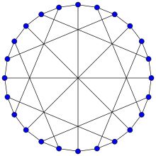
Figure 7 (The McKee graph. Image courtesy of Wikipedia.)
Below (Figure 8) is an isomorphic drawing of the graph in Figure 7 but with exactly 8 crossings. This drawing is a lot less symmetrical looking, but remember that the combinatorial symmetries of the two graphs is the same because they are isomorphic. However, as a drawing, there are symmetries of the drawing in Figure 7 that don't appear in Figure 8. For example, the vertically positioned edge in Figure 7 is a "mirror" for a reflection that maps the drawing to itself while Figure 8 has no such vertical mirror. In fact the drawing in Figure 8 has no mirror symmetry.

Figure 8 (Drawing of the McKee graph with only 8 crossings. Image courtesy of Wikipedia.)
Figure 9 is another drawing in the plane of the McKee graph with many more than 8 crossings but with appealing symmetries.

Figure 9 (Image of the McKee graph which does not achieve a minimal number of crossings but shows rotational symmetry. Image courtesy of Wikipedia.)
A graph has a collection of symmetries as a graph, which are known as automorphisms. Two isomorphic graphs have the same number of automorphisms. The number of symmetries of a drawing of a plane graph in the plane might differ from one drawing to another, and the number of symmetries of a plane drawing and a drawing which is not planar might be different. Clearly, Figures 8 and 9 do not have the same number of symmetries as drawings in the plane.
Inspired examples
When mathematicians do theoretical work, sometimes single examples serve as the inspiration for many complex ideas that evolve afterward. Sometimes small examples don't have a general property that emerges only after a certain "size" is reached. In other situations it turns out that small examples satisfy an appealing property and it is only when one gets to larger "sizes" that examples show that a statement is not universally true.
In what follows I will provide some of what I consider noteworthy historical examples of where "pretty graph theory pictures" turned the tide in helping people get breakthrough insights or helped feed interest in various topics. A further goal will be to suggest how pretty graphs inspire new ideas, new questions This often leads to additional pretty graphs.
Here is an important historic example. One of the most well known and easy-to-state problems of the emerging theory of graphs was that the conjecture that the vertices of any connected graph in the plane can be vertex-colored with 4 or fewer colors — originally the 4-color conjecture, but now the 4-color theorem. Graphs sometimes can show a high level of connectivity. Thus, a graph G is k-connected if for any pair of its vertices u and v there are at least k paths between u and v whose only vertices in common are u and v. Graphs of 3-dimensional convex polyhedra are either 3-connected, 4-connected or 5-connected.
The vertex coloring number of a graph, sometimes called the chromatic number of the graph, is the minimum number of labels (often the labels are chosen as numbers) so that two vertices joined by an edge get different colors. Figure 5 shows a graph whose chromatic number is 5 while Figure 6 shows a graph with chromatic number 2. The complete graphs show for any positive integer M no matter how large, there is a graph, the complete graph on M vertices, that requires M colors to color its vertices.
It is common for a visual image to flood a mathematician's brain with ideas sometimes not directly related to the reason the image was looked at. While we started with a problem about 4-coloring planar (plane) graphs, perhaps we might try to get insights into this problem by looking at other coloring problems. Many graphs are not planar so we might look at problems coloring the vertices of more general graphs, ones which are not necessarily planar. But for plane graphs these questions suggest themselves.
- Which plane graphs can be vertex-colored with exactly two colors?
- Which plane graphs can be vertex-colored with exactly three colors?
- Which plane graphs can be face-colored with exactly two colors?
- Which plane graphs can be face-colored with exactly three colors?
The face-coloring number of a plane graph is the number of colors needed to label the faces so that two faces that share an edge get different colors. It turns out that the four-color theorem is equivalent to the fact that a face-coloring of a plane graph can be accomplished with 4 or fewer colors, just as its vertices never need more than 4 colors to color them.
While we have not been looking at ways in which "pretty graphs" are "applicable," the problems that pretty graphs are designed to illuminate often have very appealing applications. For example, if one has a collection of committees in a legislature with members in common, one can draw a graph where each dot represents a committee, and two dots are joined by an edge if the committees they represent have a member in common. The chromatic number of this graph will be the minimum number of time slots in which the committees can be scheduled so that there is no conflict requiring a committee member to be in two places at the same time. Many applied problems can be resolved via coloring problems of different kinds, including problems related to assigning cell phone frequencies so that conversations don't conflict with one another.
The 4-color problem, now the 4-color theorem because of the work of Wolfgang Haken and Kenneth Appel, can be phrased as stating that the faces of any connected plane graph can be colored with 4 or fewer colors. This problem in turn was reduced to the question that if the plane drawing of a convex 3-dimensional polyhedron all of whose vertices had exactly 3 edges at them had a Hamilton circuit, then the faces of the graph could be colored with 4 colors. A Hamilton circuit (HC) of a graph is a tour of its vertices in a simple circuit which visits each vertex once and only once. The name for this concept honors the Irish mathematician William Rowan Hamilton (1805-1865). Note the contrast with finding an Eulerian circuit, where it was the edges that had to be toured once and only once. A Hamiltonian circuit (often there are many) in a drawing of a plane graph divides the plane into the edges on the HC, the edges in the interior of the HC and the edges exterior to the HC. The interior regions can be face-colored with two colors by selecting a region and coloring it, say, red, and the regions that are across an edge from this region (still inside the HC) are colored green. A "legal" "2-coloring" is produced in this way, and a similar argument shows the exterior regions can also be two-colored. There was a point where a claim was made that the 4-color theorem was solved because such a graph, specifically 3-valent 3-polytopal plane graphs, would have a Hamiltonian circuit. However, the great British/Canadian graph theorist William Tutte (1917-2002) was the first person to show that this was not the case by producing such a graph with 46 vertices that had no Hamilton circuit. The three "gadgets" that build up the graph are called Tutte triangles and they have the property that any HC that visits the Tutte triangles must enter at the bottom (the vertices that are at the ends of the section of the Tutte triangle that has three vertices, rather than the other sides that have 4 or 5 vertices) and exit the Tutte triangle at the "top." Can you see why organizing three Tutte triangles as shown now means that the graph in Figure 10, with an extra vertex beyond those in the three Tutte triangles, can't have an HC?
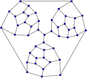
Figure 10 (A plane graph which is 3-valent and has at least three paths between any pair of distinct vertices (3-connected) which has no Hamilton circuit. Image courtesy of Wikipedia.)
Tutte's lovely example set off a search for other such plane graphs which lacked Hamilton circuits. In particular, which plane 3-connected 3-valent graph(s) have the minimal number of vertices but no HC? The answer turned out to be 38 vertices and involved the work of many people. The graph in Figure 11 is often called the Barnette–Bosák–Lederberg graph, for David Barnette, Jiraj Bosák and Joshua Lederberg, who was a Nobel Prize winner in chemistry. Lederberg's interest in HC's stemmed from a scheme he had for giving names to various molecules using Hamilton circuits to encode the information.
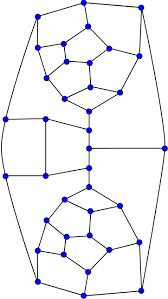
Figure 11 (A plane 3-valent 3-connected graph with a minimum number of vertices but no HC. Image courtesy of Wikipedia.)
Researchers started looking for other examples of non-Hamiltonian graphs and trying to understand the relationship between the counts on the faces of the graph and being non-Hamiltonian. Work by Grinberg showed a relatively easy way to construct many such graphs. When graphs which have different valences can be drawn in the plane it is easier to find smaller "pretty" examples of non-Hamiltonian graphs than the graphs in Figures 10 and 11. For example see the Hershel graph shown in Figure 12.
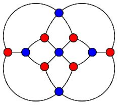
Figure 12 (Hershel graph. A bipartite plane non-Hamilton graph with a small number of vertices. Courtesy of Wikipedia)
How can one see this graph has no Hamilton circuit? Since this graph is bipartite (red vertices are only connected to blue vertices and blue vertices are only connected to red vertices) any HC of this graph would have to alternate between red and blue vertices. Thus, a Hamilton circuit in a bipartite graph would have to have equal numbers of vertices colored with the two colors. But the graph in Figure 12 has 6 red vertices and only 5 blue vertices which means it can have no HC. This graph is known named in honor of Alexander Stewart Herschel (1836-1907) due to his work on the icosian game (involving Hamilton circuits) of William Rowan Hamilton.
Another offshoot of this example from Tutte was to investigate more broadly what could be said about non-Hamiltonian polytopal graphs. For example, if a convex polyhedron has all of its vertices with the same number of edges at a vertex, it follows from Euler's polyhedral formula that this number can only be 3, 4 or 5. So, are there non-Hamilton 4-valent graphs which arise from convex 3-dimensional polyhedra? The answer is yes as shown by the "pretty graph" below due to Nico Van Cleemput and Carol Zamfirescu.

Figure 13 (A 4-valent 3-connected graph which has no Hamiltonian circuit discovered by N. Van Cleemput and C. Zamfirescu. Image courtesy of N. Van Cleemput and C. Zamfirescu.)
Having seen that the concept of finding a Hamilton circuit was so fruitful in both theoretical and applied mathematics, interest arose in graphs that have come to be called hypohamiltonian graphs. A graph is hypohamiltonian if the graph has no Hamilton circuit but deleting any vertex of the graph and the edges attached to that vertex yields a graph which is Hamiltonian. The Petersen graph (Figure 14) (named for Julius Petersen (1839-1910) has this property.
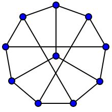
Figure 14 (The Petersen graphs is hypohamiltonian. Image courtesy of Wikipedia.)
Much harder to find are examples of planar graphs with this intriguing property. This graph (Figure 15) is a small planar graph which is hypohamiltonian.

Figure 15 (A planar hypohamiltonian graph which is also the graph of a polyhedron. Image courtesy of Wikipedia.)
This graph has a mixture of vertices of different valences. This might encourage mathematicians to study the issue of regular planar hypohamiltonian graphs, a topic which has indeed been studied.
Petersen graph
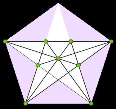
The graph below is known as the Petersen graph (different drawing from that of Figure 14) , and it is very appealing. We have seen "pieces" of this graph before but let me comment. The "outer" 5 vertices in Figure 16 form a regular convex pentagon, and the inner 5 vertices form a regular star pentagon, often called the pentagram. The corresponding vertices of the two clusters of five vertices are joined by edges. What mathematical properties does this graph have? First of all, though it does not look like the two special graphs that force the graph not to have a plane graph representation, it is, in fact, a non-planar graph.
Figure 16 (The Petersen graph. Image courtesy of Wikipedia.)
Among interesting properties of this remarkable graph are:
a. It has only 10 vertices and lacks a Hamilton circuit.
b. The edges of the graph can't be colored with exactly 3 colors even though the graph is regular of valence 3. (An edge coloring of a graph is one where each edge obtains a color and two edges that share a vertex get different colors. A remarkable theorem about edge colorings is due to the mathematician Vadim Vizing: If the maximum valence of a vertex in a graph is Δ the edge-coloring number of the graph is either Δ or Δ+1.
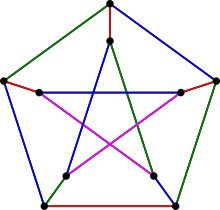
Figure 17 (An edge coloring of the Petersen graph with a minimum number of colors, namely four colors. Image courtesy of Wikipedia.)
c. The Petersen graph admits a drawing in the plane with the property that all of its edges have edge length 1.
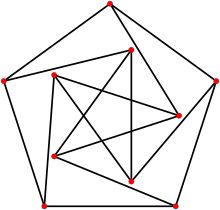
Figure 18 (An embedding of the Petersen graph in the plane where all of the edges of the graph have the same "unit" length. Image courtesy of Wikipedia.)
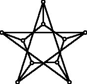
Figure 19 (Another way to embed the Petersen graph in the plane.)
It is not hard to check that the graph in Figure 19 is isomorphic to the Petersen graph. However, this drawing is particularly visually appealing. One feature of this drawing is that the places where edges meet other than vertices occurs at five points where three edges go through each of these points. In the other drawings of planar and non-planar graphs, usually there are at most two edges that go through a point that is not a crossing. This was also true for several vertices in Figure 7.
While K5 and the Petersen graph are noteworthy for a variety of problems that they directly provide some insight into, they have also inspired ideas and examples that are farther afield. Thus, Micha Perles found the inspired example of Figure 20 with 9 points and 9 lines that has the property that in any embedding of the configuration in the plane at least one point must have a coordinate that is an irrational number.
Figure 20 (Graph of the Perles configuration. Image courtesy of Wikipedia.)
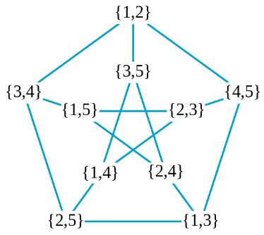
Given a collection of items making up a set, one can think about the structure of the subsets of that set. For example, consider the subsets of the set {1, 2, 3, 4, 5} which is a set of 5 elements. It is easy to see that there are 10 2-element subsets of this set. Suppose we create a graph with a vertex for each two-element subset and draw an edge between two subsets if they are disjoint, that is, have no element in common. The graph one obtains (Figure 21) is a labeled version of the Petersen graph. The idea of constructing this graph is due to Martin Kneser (1937-2004); graphs of this kind are called Kneser graphs.
Figure 21 (Kneser graph for two-element subsets of a set with 5 elements gives rise to the Petersen graph. Image courtesy of Wikipedia.)
I have tried to argue that something that is "pretty to look at" often is the starting point for something that goes beyond the "mere" inspiration and power of beauty. Mathematics is an organic subject that grows and evolves in time both in its theory and applications. Dot and line diagrams which we find beautiful will continue to have a role in this growth and evolution.
References:
Those who can access JSTOR can find some of the papers mentioned above there. For those with access, the American Mathematical Society's MathSciNet can be used to get additional bibliographic information and reviews of some of these materials. Some of the items above can be found via the ACM Portal, which also provides bibliographic services.
Many of the pretty graphs discussed above appear in a collection of images of interesting mathematical "objects," including graphs, that was prepared by David Eppstein a professor of computer science at the University of California, Ivine.
---------------------------------------------
Aldred, R., abd S. Bau, D. Holton, D., B. McKay, Nonhamiltonian 3-Connected Cubic Planar Graphs, SIAM J. Disc. Math. 13 (2000) 25-32.
Aldred, R., and B. McKay, N. Wormald, Small Hypohamiltonian Graphs, J. Combin. Math. Combin. Comput. 23 (1997) 143-152.
Araya, M. and G. Wiener, On Cubic Planar Hypohamiltonian and Hypotraceable Graphs." Elec. J. Combin. 18, 2011.
Beineke, L. and R. Wilson (eds.), Graph Connections, Oxford U. Press, Oxford, 1997.
Beineke, L. and R. Wilson (eds), Topics in Chromatic Graph Theory, Cambridge U. Press, Cambridge, 2015.
Biggs, N., and E. Lloyd, R. Wilson, Graph Theory, 1736-1936. Oxford University Press, Oxford, 1986.
Bondy, J. A. and Murty, U. S. R. Graph Theory with Applications. New York: North Holland, p. 61, 1976.
Garey, M., and D. Johnson, Computers and Intractability: A Guide to the Theory of NP-Completeness. New York: W. H. Freeman, 1983.
Gould, R., Updating the Hamiltonian problem—a survey. Journal of Graph Theory, 15 (1991) 121-157.
Lederberg, J., Hamilton Circuits of Convex Trivalent Polyhedra (up to 18 Vertices), Amer. Math. Monthly 74 (1967) 522-527.
Thomassen, C. Hypohamiltonian and Hypotraceable Graphs, Disc. Math. 9, 91-96, 1974.
Thomassen, C., On Hypohamiltonian Graphs, Disc. Math. 10, 383-390, 1974.
Thomassen, C. Planar and infinite hypohamiltonian and hypotraceable Graphs, Disc. Math 14, 377-389, 1976.
Tutte, W. , On Hamiltonian Circuits. J. London Math. Soc. 21 (1946) 98-101.
Van Cleemput, N. and C. Zamfirescu, Regular non-hamiltonian polyhedral graphs, Applied Mathematics and Computation, 338 (2018) 192-206
Zamfirescu, C., On hypohamiltonian and almost hypohamiltonian graphs, Journal of Graph Theory 79 (2015) 63-81
Joseph Malkevitch
York College (CUNY)
Email Joseph Malkevitch