Pooling strategies for COVID-19 testing
How could 10 tests yield accurate results for 100 patients?
While the COVID-19 pandemic has brought tragedy and disruption, it has also provided a unique opportunity for mathematics to play an important and visible role in addressing a pressing issue facing our society.
By now, it's well understood that testing is a crucial component of any effective strategy to control the spread of the SARS-CoV-2 coronavirus. Countries that have developed effective testing regimens have been able, to a greater degree, to resume normal activities, while those with inadequate testing have seen the coronavirus persist at dangerously high levels.
Developing an effective testing strategy means confronting some important challenges. One is producing and administering enough tests to form an accurate picture of the current state of the virus' spread. This means having an adequate number of trained health professionals to collect and process samples along with an adequate supply of reagents and testing machines. Furthermore, results must be available promptly. A person is who unknowingly infected can transmit the virus to many others in a week, so results need to be available in a period of days or even hours.
One way to address these challenges of limited resources and limited time is to combine samples from many patients into testing pools strategically rather than testing samples from each individual patient separately. Indeed, some well-designed pooling strategies can decrease the number of required tests by a factor of ten; that is, it is possible to effectively test, say, 100 patients with a total of 10 tests.
On first thought, it may seem like we're getting something from nothing. How could 10 tests yield accurate results for 100 patients? This column will describe how some mathematical ideas from compressed sensing theory provide the key.
One of the interesting features of the COVID-19 pandemic is the rate at which we are learning about it. The public is seeing science done in public view and in real time, and new findings sometimes cause us to amend earlier recommendations and behaviors. This has made the job of communicating scientific findings especially tricky. So while some of what's in this article may require updating in the near future, our aim is rather to focus on mathematical issues that should remain relevant and trust the reader to update as appropriate.
Some simple pooling strategies
While the SARS-CoV-2 virus is new, the problem of testing individuals in a large population is not. Our story begins in 1943 when Robert Dorfman proposed the following simple method for identifying syphilitic men called up for induction through the war time draft.
Suppose we have samples from, say, 100 patients. Rather than testing each of the samples individually, Dorfman suggested grouping them into 10 pools of 10 each and testing each pool.
If the test result of a pool is negative, we conclude that everyone in that pool is free of infection. If a pool tests positively, then we test each individual in the pool.
In the situation illustrated above, two of the 100 samples are infected, so we perform a total of 30 tests to identify them: 10 tests for the original 10 pools followed by 20 tests for each member of the two infected pools. Here, the number of tests performed is 30% of the number required had we tested each individual separately.
Of course, there are situations where this strategy is disadvantageous. If there is an infected person in every pool, we end up performing the original 10 tests and follow up by then testing each individual. This means we perform 110 tests, more than if we had just tested everyone separately.
What's important is the prevalence $p$ of the infection, the expected fraction of infected individuals we expect to find or the probability that a random individual is infected. If the prevalence is low, it seems reasonable that Dorfman's strategy can lead to a reduction in the number of tests we expect to perform. As the prevalence grows, however, it may no longer be effective.
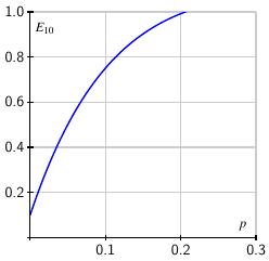 It's not too hard to find how the expected number of tests per person varies with the prevalence. If we arrange $k^2$ samples into $k$ pools of $k$ samples each, then the expected number of tests per person is $$ E_k = \frac1k + (1-(1-p)^k). $$ When $k=10$, the expected number $E_{10}$ is shown on the right. Of course, testing each individual separately means we use one test per person so Dorfman's strategy loses its advantage when $E_k\geq 1$. As the graph shows, when $p>0.2$, meaning there are more than 20 infections per 100 people, we are better off testing each individual.
Fortunately, the prevalence of SARS-CoV-2 infections is relatively low in the general population. As the fall semester began, my university initiated a randomized testing program that showed the prevalence in the campus community to be around $p\approx 0.01$. Concern is setting in now that that number is closer to 0.04. In any case, we will assume that the prevalence of infected individuals in our population is low enough to make pooling a viable strategy.
Of course, no test is perfect. It's possible, for instance, that an infected sample will yield a negative test result. It's typical to characterize the efficacy of a particular testing protocol using two measures: sensitivity and specificity. The sensitivity measures the probability that a test returns a positive result for an infected sample. Similarly, the specificity measures the probability that a test returns a negative result when the sample is not infected. Ideally, both of these numbers are near 100%.
Using Dorfman's pooling method, the price we pay for lowering the expected number of tests below one is a decrease in sensitivity. Identifying an infected sample in this two-step process requires the test to correctly return a positive result both times we test it. Therefore, if $S_e$ is the sensitivity of a single test, Dorfman's method has a sensitivity of $S_e^2$. For example, a test with a sensitivity of 95% yields a sensitivity around 90% when tests are pooled.
There is, however, an increase in the specificity. If a sample is not infected, testing a second time increases the chance that we detect it as such. One can show that if the sensitivity and specificity are around 95% and the prevalence at 1%, then pooling 10 samples, as shown above, raises the specificity to around 99%.
Some modifications of Dorfman's method
It's possible to imagine modifying Dorfman's method in several ways. For instance, once we have identified the infected pools in the first round of tests, we could apply a pooling strategy on the smaller set of samples that still require testing.
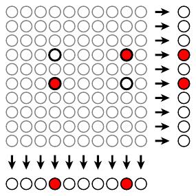
A second possibility is illustrated below where 100 samples are imagined in a square $10\times10$ array. Each sample is included in two pools according to its row and column so that a total of 20 tests are performed in the first round. In the illustration, the two infected samples lead to positive results in four of the pools, two rows and two columns.
We know that the infected samples appear at the intersection of these two rows and two columns, which leads to a total of four tests in the second round. Once again, it's possible to express $E_k$, the number of expected tests per individual in terms of the prevalence $p$. If we have $k^2$ tests arranged in a $k\times k$ array, we see that $$ E_k =\frac2k + p + (1-p)(1-(1-p)^{k-1}, $$ if we assume that the sensitivity and specificity are 100%.
 The graph at right shows the expected number of tests using the two-dimensional array, assuming $k=10$, in red with the result using Dorfman's original method in blue. As can be seen, the expected number of tests is greater using the two-dimensional approach since we invest twice as many tests in the first round of testing. However each sample is included in two tests in the initial round. For an infected sample to be misidentified, both tests would have to return negative results. This means that the two-dimensional approach is desirable because the sensitivity of this strategy is greater than the sensitivity of the individual tests and we still lower the expected number of tests when the prevalence is low.
While it is important to consider the impact that any pooling strategy has on these important measures, our focus will, for the most part, take us away from discussions of specificity and sensitivity. See this recent Feature column for a deep dive into their relevance.
Theoretical limits
There has been some theoretical work on the range of prevalence values over which pooling strategies are advantageous. In the language of information theory, we can consider a sequence of test results as an information source having entropy $I(p) = -p\log_2(p) - (1-p)\log_2(1-p)$. In this framework, a pooling strategy can be seen as an encoding of the source to effectively compress the information generated.
 Sobel and Groll showed that $E$, the expected number of tests per person, for any effective pooling method must satisfy $E \geq I(p)$. On the right is shown this theoretical limit in red along with the expected number of tests under the Dorfman method with $k=10$.
Further work by Ungar showed that when the prevalence grows above the threshold $p\geq (3-\sqrt{5})/2 \approx 38\%$, then we cannot find a pooling strategy that is better than simply testing everyone individually.
RT-qPCR testing
While there are several different tests for the SARS-CoV-2 virus, at this time, the RT-qPCR test is considered the "gold standard." In addition to its intrinsic interest, learning how this test works will help us understand the pooling strategies we will consider next.
A sample is collected from a patient, often through a nasal swab, and dispersed in a liquid medium. The test begins by converting the virus' RNA molecules into complementary DNA through a process known as reverse transcription (RT). A sequence of amplification cycles, known as quantitative polymerase chain reaction (qPCR) then begins. Each cycle consists of three steps:
-
The liquid is heated close to boiling so that the transcribed DNA denatures into two separate strands.
-
Next the liquid is cooled so that a primer, which has been added to the liquid, attaches to a DNA strand along a specific sequence of 100-200 nucleotides. This sequence characterizes the complementary DNA of the SARS-CoV-2 virus and is long enough to uniquely identify it. This guarantees that the test has a high sensitivity. Attached to the primer is a fluorescent marker.
-
In a final warming phase, additional nucleotides attach to the primer to complete a copy of the complementary DNA molecule.
Through one of these cycles, the number of DNA molecules is essentially doubled.
The RT-qPCR test takes the sample through 30-40 amplification cycles resulting in a significant increase in the number of DNA molecules, each of which has an attached fluorescent marker. After each cycle, we can measure the amount of fluorescence and translate it into a measure of the number of DNA molecules that have originated from the virus.
The fluorescence, as it depends on the number of cycles, is shown below. A sample with a relatively high viral load will show significant fluorescence at an early cycle. The curves below represent different samples and show how the measured fluorescence grows through the amplification cycles. Moving to the right, each curve is associated with a ten-fold decrease in the initial viral load of the sample. Taken together, these curves represent a range of a million-fold decrease in the viral load. In fact, the test is sensitive enough to detect a mere 10 virus particles in a sample.
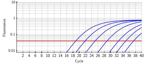
The FDA has established a threshold, shown as the red horizontal line, above which we can conclude that the SARS-CoV-2 virus is present in the original sample. However, the test provides more than a binary positive/negative result; by matching the fluorescence curve from a particular sample to the curves above, we can infer the viral load present in the original sample. In this way, the test provides a quantitative measure of the viral load that we will soon use in developing a pooling method.
Pooling samples from several individuals, only one of whom is infected, will dilute the infected sample. The effect is simply that the fluorescence response crosses the FDA threshold in a later cycle. There is a limit, however. Because noise can creep into the fluorescence readings around cycle 40, FDA standards state that only results from the first 39 cycles are valid.
Recent studies by Bilder and Yelin et al investigated the practical limits of pooling samples in the RT-qPCR test and found that a single infected sample can be reliably detected in a pool of up to 32. (A recent study by the CDC, however, raises concerns about detecting the virus using the RT-qPCR test past the 33rd amplification cycle. )
Non-adaptive testing strategies
Dorfman's pooling method and its variants described above are known as adaptive methods because they begin with an initial round of tests and use those results to determine how to proceed with a second round. Since the RT-qPCR test requires 3 - 4 hours to complete, the second round of testing causes a delay in obtaining results and ties up testing facilities and personnel. A non-adaptive method, one that produces results for a group of individuals in a single round of tests, would be preferable.
Several non-adaptive methods have recently been proposed and are even now in use, such as P-BEST. The mathematical ideas underlying these various methods are quite similar. We will focus on one called Tapestry.
We first collect samples from $N$ individuals and denote the viral loads of each sample by $x_j$. We then form these samples into $T$ pools in a manner to be explained a little later. This leads to a pooling matrix $A_i^j$ where $A_i^j = 1$ if the sample from individual $j$ is present in the $i^{th}$ test and 0 otherwise. The total viral load in the $i^{th}$ test is then $$ y_i = \sum_{j} A_i^j x_j, $$ which can be measured by the RT-qPCR test. In practice, there will be some uncertainty in measuring $y_i$, but it can be dealt with in the theoretical framework we are describing.
Now we have a linear algebra problem. We can express the $T$ equations that result from each test as $$ \yvec = A\xvec, $$ where $\yvec$ is the known vector of test results, $A$ is the $T\times N$ pooling matrix, and $\xvec$ is the unknown vector of viral loads obtained from the patients.
Because $T\lt N$, this is an under-determined system of equations, which means that we cannot generally expect to solve for the vector $\xvec$. However, we have some additional information: because we are assuming that the prevalence $p$ is low, the vector $\xvec$ will be sparse, which means that most of its entries are zero. This is the key observation on which all existing non-adaptive pooling methods rely.
It turns out that this problem has been extensively studied within the area of compressed sensing, a collection of techniques in signal processing that allow one to reconstruct a sparse signal from a small number of observations. Here is an outline of some important ideas.
First, we will have occassion to consider a couple of different measures of the size of a vector.
-
First, $\norm{\zvec}{0}$ is the number of nonzero entries in the vector $\zvec$. Because the prevalence of SARS-CoV-2 positive samples is expected to be small, we are looking for a solution to the equation $\yvec=A\xvec$ where $\norm{\xvec}{0}$ is small.
-
The 1-norm is $$ \norm{\zvec}{1} = \sum_j~|z_j|, $$
-
and the 2-norm is the usual Euclidean length: $$ \norm{\zvec}{2} = \sqrt{\sum_j z_j^2} $$
Remember that an isometry is a linear transformation that preserves the length of vectors. With the usual Euclidean length of a vector $\zvec$ written as $||\zvec||_2$, then the matrix $M$ defines an isometry if $||M\zvec||_2 = ||\zvec||_2$ for all vectors $\zvec$. The columns of such a matrix form an orthonormal set.
We will construct our pooling matrix $A$ so that it satisfies a restricted isometry property (RIP), which essentially means that small subsets of the columns of $A$ are almost orthonormal. More specifically, if $R$ is a subset of $\{1,2,\ldots, N\}$, we denote by $A^R$ the matrix formed by pulling out the columns of $A$ labelled by $R$; for instance, $A^{\{2,5\}}$ is the matrix formed from the second and fifth columns of $A$. For a positive integer $S$, we define a constant $\delta_S$ such that $$ (1-\delta_S)||\xvec||_2 \leq ||A^R\xvec||_2 \leq (1+\delta_S)||\xvec||_2 $$ for any set $R$ whose cardinality is no more than $S$. If $\delta_S = 0$, then the matrices $A^R$ are isometries, which would imply that the columns of $A^R$ are orthonormal. More generally, the idea is that when $\delta_S$ is small, then the columns of $A^R$ are close to being orthonormal.
Let's see how we can use these constants $\delta_S$.
Because we are assuming that the prevalence $p$ is low, we know that $\xvec$, the vector of viral loads, is sparse. We will show that a sufficiently sparse solution to $\yvec = A\xvec$ is unique.
For instance, suppose that $\delta_{2S} \lt 1$, that $\xvec_1$ and $\xvec_2$ are two sparse solutions to the equation $\yvec = A\xvec$, and that $\norm{\xvec_1}{0}, \norm{\xvec_1}{0} \leq S$. The last condition means that $\xvec_1$ and $\xvec_2$ are sparse in the sense that they have fewer than $S$ nonzero components.
Now it follows that $A\xvec_1 = A\xvec_2 = \yvec$ so that $A(\xvec_1-\xvec_2) = 0$. In fact, if $R$ consists of the indices for which the components of $\xvec_1-\xvec_2$ are nonzero, then $A^R(\xvec_1-\xvec_2) = 0$.
But we know that the cardinality of $R$ equals $\norm{\xvec_1-\xvec_2}{0} \leq 2S$, which tells us that $$ 0 = ||A^R(\xvec_1-\xvec_2)||_2 \geq (1-\delta_{2S})||\xvec_1-\xvec_2||_2. $$ Because $\delta_{2S}\lt 1$, we know that that $\xvec_1 - \xvec = 0$ or $\xvec_1 = \xvec_2$.
Therefore, if $\delta_{2S} \lt 1$, any solution to $\yvec=A\xvec$ with $\norm{\xvec}{0} \leq S$ is unique; that is, any sufficiently sparse solution is unique.
Now that we have seen a condition that implies that sparse solutions are unique, we need to explain how we can find sparse solutions. Candès and Tao show, assuming $\delta_S + \delta_{2S} + \delta_{3S} \lt 1$, how we can find a sparse solution to $\yvec = A\xvec$ with $\norm{\xvec}{0} \leq S$ by minimizing: $$ \min \norm{\xvec}{1} ~~~\text{subject to}~~~ \yvec = A\xvec. $$ This is a convex optimization problem, and there are standard techniques for finding the minimum.
Why is it reasonable to think that minimizing $\norm{x}{1}$ will lead to a sparse solution? Let's think visually about the case where $\xvec$ is a 2-dimensional vector. The set of all $\xvec$ satisfying $\norm{\xvec}{1} = |x_1| + |x_2| \leq C$ for some constant $C$ is the shaded set below:
Notice that the corners of this set fall on the coordinate axes where some of the components are zero. If we now consider solutions to $\yvec=A\xvec$, seen as the line below, we see that the solutions where $\norm{\xvec}{1}$ is minimal fall on the coordinates axes. This forces some of the components of $\xvec$ to be zero and results in a sparse solution.
This technique is related to one called the lasso (least absolute shrinkage and selection operator), which is well known in data science where it is used to eliminate unnecessary features from a data set.
All that remains is for us to find a pooling matrix $A$ that satisfies $\delta_{S} + \delta_{2S} + \delta_{3S} \lt 1$ for some $S$ large enough to find vectors $\xvec$ whose sparsity $\norm{\xvec}{0}$ is consistent with the expected prevalence. There are several ways to do this. Indeed, a matrix chosen at random will work with high probability, but the application to pooling SARS-CoV-2 samples that we have in mind leads us to ask that $A$ satisfy some additional properties.
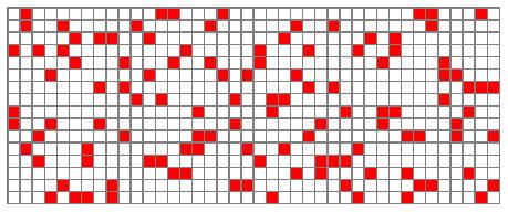
The Tapestry method uses a pooling matrix $A$ formed from a Steiner triple system, an object studied in combinatorial design theory. For instance, one of Tapestry's pooling matrices is shown below, where red represents a 1 and white a 0.
This is a $16\times40$ matrix, which means that we perform 16 tests on 40 individuals. Notice that each individual's sample appears in 3 tests. This is a relatively low number, which means that the viral load in a sample is not divided too much and that, in the laboratory, time spent pipetting the samples is minimzed. Each test consists of samples from about eight patients, well below the maximum of 32 needed for reliable RT-qPCR readings.
It is also important to note that two samples appear together in at most one test. Therefore, if $A^j$ is the $j^{th}$ column of $A$, it follows that the dot product $A^j\cdot A^k = 0$ or $1$. This means that two columns are either orthogonal or span an angle of $\arccos(1/3) \approx 70^\circ$. If we scale $A$ by $1/\sqrt{3}$, we therefore obtain a matrix whose columns are almost orthonormal and from which we can derive the required condition, $\delta_S + \delta_{2S} + \delta_{3S} \lt 1$ for some sufficiently large value of $S$.
There is an additional simplification we can apply. For instance, if we have a sample $x_j$ that produces a negative result $y_i=0$ in at least one test in which it is included, then we can conclude that $x_j = 0$. This means that we can remove the component $x_j$ from the vector $\xvec$ and the column $A^j$ from the matrix $A$. Removing all these sure negatives often leads to a dramatic simplication in the convex optimization problem.
Tapestry has created a variety of pooling matrices that can be deployed across a range of prevalences. For instance, a $45\times 105$ pooling matrix, which means we perform 45 tests on 105 individuals, is appropriate when the prevalence is roughly 10%, a relatively high prevalence.
However, there is also a $93\times 961$ pooling matrix that is appropriate for use when the prevalence is around 1%. Here we perform 93 tests on 961 patients in pools of size 32, which means we can test about 10 times the number of patients with a given number of tests. This is a dramatic improvement over performing single tests on individual samples.
If the prevalence turns out to be too high for the pooling matrix used, the Tapestry algorithm detects it and fails gracefully.
Along with non-adaptive methods comes an increase in the complexity of their implementation. This is especially concerning since reliability and speed are crucial. For this reason, the Tapestry team built an Android app that guides a laboratory technician though the pipetting process, receives the test results $y_i$, and solves for the resulting viral loads $x_j$ returning a list of positive samples.
Using both simulated and actual lab data, the authors of Tapestry studied the sensitivity and specificity of their algorithm and found that it performs well. They also compared the number of tests Tapestry performs with Dorfman's adaptive method and found that Tapestry requires many fewer tests, often several times fewer, in addition to finishing in a single round.
Summary
As we've seen here, non-adaptive pooling provides a significant opportunity to improve our testing capacity by increasing the number of samples we can test, decreasing the amount of time it takes to obtain results, and decreasing the costs of testing. These improvements can play an important role in a wider effort to test, trace, and isolate infected patients and hence control the spread of the coronavirus.
In addition, the FDA recently gave emergency use authorization for the use of these ideas. Not only is there a practical framework for deploying the Tapestry method, made possible by their Android app, it's now legal to do so.
Interestingly, the mathematics used here already existed before the COVID-19 pandemic. Dating back to Dorfman's original work of 1943, group pooling strategies have continued to evolve over the years. Indeed, the team of Shental et al. introduced P-BEST, their SARS-CoV-2 pooling strategy, as an extension of their earlier work to detect rare alleles associated to some diseases.
Thanks
Mike Breen, recently of the AMS Public Awareness Office, oversaw the publication of the monthly Feature Column for many years. Mike retired in August 2020, and I'd like to thank him for his leadership, good judgment, and never-failing humor.
References
-
David Donoho. A Mathematical Data Scientist's perspective on Covid-19 Testing Scale-up. SIAM Mathematics of Data Science Distinguished Lecture Series. June 29, 2020.
Donoho's talk is a wonderful introduction to and overview of the problem, several approaches to it, and the workings of the scientific community.
-
Claudio M. Verdun et al. Group testing for SARS-CoV-2 allows for up to 10-fold efficiency increase across realistic scenarios and testing strategies.
This survey article provides a good overview of Dorfman's method and similar techniques.
-
Chris Bilder. Group Testing Research.
Bilder was prolific in the area of group testing before (and after) the COVID-19 pandemic, and this page has many good resources, including this page of Shiny apps.
-
Idan Yelin et al. Evaluation of COVID-19 RT-qPCR Test in Multi sample Pools. Clinical Infectious Diseases, May 2020.
-
Milton Sobel and Phyllis A. Groll. Group testing to eliminate efficiently all defectives in a binomial sample. Bell System Technical Journal, Vol. 38, Issue 5, Sep 1959. Pages 1179–1252.
-
Peter Ungar. The cutoff point for group testing. Communications on Pure and Applied Mathematics, Vol. 13, Issue 1, Feb 1960. Pages 49-54.
-
Tapestry Pooling home page.
-
Ghosh et al. Tapestry: A Single-Round Smart Pooling Technique for COVID-19 Testing
This paper and the next outline the Tapestry method.
-
Ghosh et al. A Compressed Sensing Approach to Group-testing for COVID-19 Detection.
-
N. Shental et al. Efficient high-throughput SARS-CoV-2 testing to detect asymptomatic carriers.
This article and the next describe the P-BEST technique.
-
Noam Shental, Amnon Amir, and Or Zuk. Identification of rare alleles and their carriers using compressed se(que)nsing. Nucleic Acids Research, 2010, Vol. 38, No. 19.
-
David L. Donoho. Compressed Sensing. IEEE Transactions on Information Theory. Vol. 52, No. 4, April 2006.
-
Emamnuel J. Candès. Compressive sampling. Proceedings of the international congress of mathematicians. Vol. 2, 2006. Pages 1433-1452.
-
Emmanuel Candès, Justin Romberg, and Terence Tao. Stable Signal Recovery from Incomplete and Inaccurate Measurements. Communications in Pure and Applied Mathematics. Vol. 59, Issue 8, August 2006. Pages 1207-1223.
-
Emmanuel Candès and Terence Tao. Decoding by Linear Programming. IEEE Transactions on Information Theory. Vol. 51, Issue 12, Dec. 2005. Pages 4203-4215.
-
Chun Lam Chan, Pak Hou Che and Sidharth Jaggi. Non-adaptive probabilistic group testing with noisy measurements: Near-optimal bounds with efficient algorithms. 2011 49th Annual Allerton Conference on Communication, Control, and Computing (Allerton). Monticello, IL, 2011. Pages 1832-1839.
-
Steiner system. Wikipedia page.
 David Austin