The Center of Population of the United States

Posted February 2005.

I'll discuss why finding the center is problematic and suggest
an alternative method for the Census Bureau to use. . . .

David Austin
Grand Valley State University
david at merganser.math.gvsu.edu

Mail to a friend

Print this article

Introduction

The United States Constitution established a national census in order to apportion, among other things, congressional representatives. The first U.S. census, conducted in 1790 under the supervision of Secretary of State Thomas Jefferson, charged federal marshals with visiting every household to obtain six pieces of information: the name of the household and the number of free white males older than 16, free white males younger than 16, free white females, other free persons, and slaves. That census counted 3.9 million people and required 18 months to complete.

Over time, it became clear that more detailed statistical information about the population would help to formulate better policy, and accordingly the census began to collect additional information about, say, manufacturing, crime, taxation, and pauperism. Combined with a growing population, this made the task of collecting and analyzing the information more formidable. For instance, the 1880 census, which counted a population of 50.2 million, collected such a large amount of data that it took ten years to tabulate and publish the results. This problem led Herman Hollerith, a one-time census statistician, to develop both a machine to record census data on punch cards and a machine, shown at the right, to read the cards and convert the data into electrical impulses thus allowing the data to be counted mechanically. Hollerith's machine, first used in the 1890 census, trimmed the time for counting the population of nearly 63 million from an expected two years to three months and saved an estimated $5 million. After leaving the Census Bureau, Hollerith founded the Tabulating Machine Company, which after a merger and Hollerith's retirement, was renamed the International Business Machines Corporation.

However, once the data from a census has been tabulated, the daunting task of analyzing it and presenting it in a meaningful way remains. For example, the population distribution of the conterminous 48 states in the 2000 census may be represented as shown below. Regions with a higher population density are shaded in a darker blue. (This map is drawn in the Albers equal-area projection.)

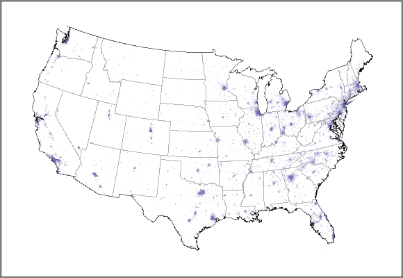
If we look at a similar map for the 1990 census, how could we compare the two maps and derive meaningful conclusions? For instance, the maps would indicate that the population is generally moving west and south, but we would like to have an efficient way to quantify how fast and in what direction the population is moving. To that end, the U.S. Census Bureau computes and publishes a location called the "mean center of population" for the U.S.. Designed to represent the average location of all residents of the U.S., this location is described by the Census Bureau as follows:

The concept of the center of population as used by the U.S. Census Bureau is that of a balance point. That is, the center of population is the point at which an imaginary, weightless, rigid, and flat (no elevation effects) surface representation of the 48 conterminous states and the District of Columbia (or 50 states as appropriate to the computation) would balance if weights of identical size were placed on it so that each weight represented the location of one person.

This seems like a natural location for it has a simple intuitive meaning that condenses the population distribution into a single point that may be tracked from one census to the next.

To compute this center, the geographic area of the U.S. is first broken into over 66,300 smaller pieces called "tracts." The tracts are designed so that, as much as possible, the population residing in a tract has rather homogeneous characteristics such as economic status and living conditions. Ideally, the population of a tract is about 1500 to 8000, which means that the geographic areas of the tracts vary considerably. As the tracts are meant to persist from one census to the next, the requirement of homogeneity creates a relatively stable population group that allows for meaningful comparisons across time. The population distribution shown above was created by shading each of the tracts according to its population density.

Typically speaking, however, the tracts are small enough that they may be thought of as a single point on the Earth's surface described by a latitude $\phi$ and a longitude $\lambda$ . Recall that latitude is an angular measure of the distance from a point on the Earth's surface to the equator while longitude measures the angular distance from the Prime Meridian. The position of a tract is denoted by $(\phi_i,\lambda_i)$ and its population $w_i$ .

The Census Bureau then defines the center of population as being given by

$\bar{\phi}=\frac{\sum_iw_i\phi_i}{\sum_i w_i},\qquad \bar{\lambda}=\frac{\sum_iw_i\lambda_i\cos\phi_i}{\sum_i w_i\cos\phi_i}.$

Applying these formulas to the data from the 2000 Census locates the center of population at

$\bar{\phi}=\hbox{37N42},\quad\bar{\lambda}=\hbox{91W34},$

near the town of Edgar Springs, Missouri.

The position of this center receives considerable public attention; Steelville, Missouri, the town nearest the location designated as the center in the 1990 Census, placed a marker in its city park in recognition.

A few years ago, my colleague Ed Aboufadel pointed out these formulas to me and expressed his concern that they did not accomplish the reasonable aim that the Census Bureau set for itself. In this note, I'll discuss why these formulas are problematic and suggest an alternative method for the Census Bureau to use.

Balancing points

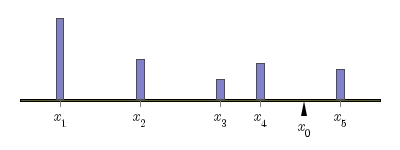Since the aim of the Census Bureau is to describe a balancing point, let's begin with a discussion of balancing points. The simplest situation is familiar to anyone who has played on a teeter-totter: We'll imagine that a series of weights are laid out on a one-dimensional board supported at one point and consider the tendency of the board to rotate about this support. Each block will have position $x_i$ and mass $m_i$ . Imagine also that the support is located at $x_0$ . A physical principle called the law of moments says that the tendency of the board to rotate is measured by the moment about the point $x_0$ :

$M_{x_0}=\sum_im_i(x_i-x_0)$

This is also familiar to anyone who has used a lever and fulcrum: A smaller mass, located sufficiently far from the fulcrum, can lift a larger mass.

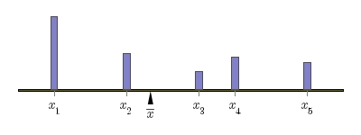The balancing point $\bar{x}$ occurs at the point where the moment $M_{\bar{x}}=\sum_im_i(x_i-\bar{x}) = 0$ . After suitably rearranging this expression, we find that

$\bar{x}=\frac{\sum_im_ix_i}{\sum_im_i}.$

Let's think about this expression within the context of population. Suppose that a collection of $ N $ people, all of whom have the same mass, are now standing along the board and that the number of people standing at $x_i$ is $w_i$ . We see that the the balancing point is really given by simply averaging the $ x $ coordinates of all the people:

$\bar{x}=\frac{\sum_iw_ix_i}{\sum_iw_i} =\frac{\overbrace{x_1+\ldots+x_1}^{w_1 \hbox{ times}}+\overbrace{x_2+\ldots+x_2} ^{w_2\hbox{ times}} +\ldots+\overbrace{x_n+\ldots+x_n}^{w_n\hbox{times}}}{N}$

The situation in which we have a collection of blocks laid out on a two-dimensional board is really no more difficult. Here, each block is described by its mass $m_i$ and its position $ (x_i,y_i) $ .

If the balancing point is $(\bar{x},\bar{y})$ , we see, by looking at the board from along the $ y $ axis, that the board should balance about $\bar{x}$ , and, by looking at the board from along the $ x $ axis, that the board should balance about $\bar{y}$ .

This leads to the expressions

$\bar{x}=\frac{\sum_i m_ix_i}{\sum_im_i},\qquad \bar{y}=\frac{\sum_i m_iy_i}{\sum_im_i}$

or within the context of population

$\bar{x}=\frac{\sum_i w_ix_i}{\sum_iw_i},\qquad \bar{y}=\frac{\sum_i w_iy_i}{\sum_iw_i}$

These expressions now begin to look something like the formulas used by the Census Bureau. In fact, it can be seen that the expression for $\bar{\phi}=\frac{\sum_iw_i\phi_i}{\sum_iw_i}$ is simply the average latitude. But what about the expression for $\bar{\lambda}$ ?

Interpreting the Census Bureau's formula

The Sanson-Flamsteed, or sinusoidal, projection is a commonly used means of creating maps of the Earth's surface. Here, one chooses a central meridian, or a line of longitude $\lambda_0$ , that will serve as the horizontal center of the map. Then a point with latitude $\phi$ and longitude $\lambda$ is mapped to a point in the $x$-$y$ plane by

$x=(\lambda-\lambda_0)\cos\phi,\qquad y=\phi$

Using the Prime Meridian as the central meridian produces a map of the world as shown below:

This map projection has several useful properties:

Lines of constant latitude are mapped into horizontal lines making the projection useful, for example, in meterology as it allows regions at the same latitude to be compared easily.
The length of parallels of latitude are represented in the correct proportion to one another.
Regions with equal area on the Earth's surface appear with equal area on the map.

The formula used to compute the center of population of the U.S. may be interpreted in terms of the Sanson-Flamsteed projection.

$\bar{\phi}=\frac{\sum_iw_i\phi_i}{\sum_i w_i},\qquad \bar{\lambda}=\frac{\sum_iw_i\lambda_i\cos\phi_i}{\sum_i w_i\cos\phi_i}.$

As noted by F. E. Barmore (in the references below), if the longitude $\bar{\lambda}$ determined by the Census is used as the central meridian in a Sanson-Flamsteed projection, the balancing point will occur along the $y$ axis at the point $(0,\bar{\phi})$ . To see this, consider

$\begin{eqnarray*} \bar{x}&=&\frac{\sum_iw_ix_i}{\sum_iw_i}\\ &=& \frac{\sum_iw_i(\lambda_i-\bar{\lambda})\cos\phi_i} {\sum_iw_i}\\ &=& \frac{\sum_iw_i\lambda_i\cos\phi_i- \bar{\lambda}\sum_iw_i\cos\phi_i}{\sum_iw_i}\\ &=& \frac{\sum_iw_i\lambda_i\cos\phi_i- \sum_iw_i\lambda_i\cos\phi_i}{\sum_iw_i}\\ &=& 0 \end{eqnarray*}$

Shown below is the population distribution of the conterminous 48 states from the 2000 Census, this time drawn in the Sanson-Flamsteed projection where the central meridian is $\bar{\lambda}$ = 91W34. The center of population computed by the Census Bureau is indicated in red. The center is the actual balancing point of the distribution as drawn on this flat map.

Representing the earth on a flat map

It is a fact well known to map-makers, however, that any map of the earth drawn on a flat surface necessarily distorts the distances between points. This is relevant for us since the computation of a balancing point, as explained above, relies on an understanding of distance.

This property of maps follows from a remarkable theorem due to Carl Friedrich Gauss, which he called his Theorema Egregium or "notable theorem." The statement of this theorem relies on an understanding of what we now call Gaussian curvature. The aim of this quantity is to measure how a two-dimensional surface residing in three-dimensional space is curved. Its definition is simple enough to understand.

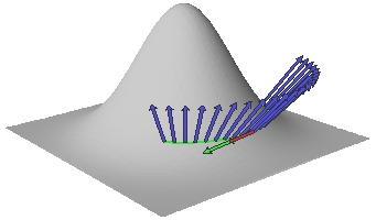
First, consider a surface sitting in three-dimensional space and let ${\bf N}$ be a vector field that has unit length and is everywhere normal (perpendicular) to the surface. Now suppose that we are standing at a point $p$ on the surface. We can define the Gaussian curvature $K(p)$ as a real number that measures something about how the surface is curved in space. To do this, we will imagine moving along a path through the point $p$ with velocity ${\bf v}$ . As we move along this path, the normal vector will also change. In particular, we can define $S_{p}({\bf v})$ to be the vector that measures the derivative of ${\bf N}$ as we move along the path. This is shown in the figure to the right.

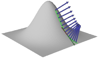
In the case that $S_{p}({\bf v})$ is parallel to ${\bf v}$ , we call ${\bf v}$ a principal direction. This means that there is a scalar $k_{\bf v}$ , called the principal curvature, such that

$S_p({\bf v}) = k_{\bf v}{\bf v}$

As shown below, there are always two orthogonal principal directions ${\bf v}$ and ${\bf w}$ , and the Gaussian curvature is defined to be

$K(p)=k_{\bf v}k_{\bf w}.$

To say this more succintly, one notices that the shape operator $S_p$ is a linear transformation from the tangent space at $p$ to itself. In fact, this linear transformation is symmetric and the Gaussian curvature is merely the product of its two eigenvalues. The average of the two eigenvalues is known as the mean curvature and is a useful measurement in other contexts.

Here are a few examples to consider:

Plane: Since the normal vector field ${\bf N}$ is constant on the plane, every direction is a principal direction with principal curvature 0. Therefore at every point .
Cylinder: As shown, there are two principal directions, one of whose principal curvature is zero. Therefore, at every point .
Sphere: Every direction is a principal direction with principal curvature where is the radius of the sphere. Therefore, at every point .

With this notion of curvature understood, we may now state Gauss's theorem:

Theorema Egregium: Any function between surfaces that preserves the distance between nearby points must also preserve the Gaussian curvature.

What does this have to do with maps? A map may be thought of as a function from the sphere (or at least a portion of the sphere) to a plane. Since the sphere and plane have different curvatures, Gauss's theorem tells us there can be no distance-preserving map. That is, when we draw maps of the Earth's surface, we must inevitably distort some distances. This has some bearing on our problem: The computation of a balancing point, as we have seen, depends on measuring distances. Since any map distorts distances, we will generally not find a balancing point by first mapping the Earth onto a flat surface and then computing.

Aside from its application to map-making, the Theorema Egregium is extremely important in geometry for it implies that Gaussian curvature depends only on how distances are measured on the surface and not, as it would appear from the definition, on how the surface sits inside three-dimensional space. To illustrate this point, think of how a poster can be rolled into a cylinder. If distances measured on the surface were distorted, tears or wrinkles would appear in the poster, but there are none. Therefore the rolled-up poster, even though it is curled, still has zero curvature.

Furthermore, since distances on the surface can be measured without referring to the surrounding space, curvature is a quantity that can be detected by inhabitants of the surface. For instance, if we stand at point $p$ , the set of points whose distance from us is $\rho$ forms a curve whose length we may call $C_\rho$ . For the plane, of course, we know that this set of points is a circle and that $C_\rho=2\pi\rho$ . For a surface, however, the curvature at $p$ may be found as $ -3 $ times the second derivative of $C_\rho/2\pi\rho$ at $\rho=0$ . In a similar way, cosmologists, say, may profitably work with the curvature of the universe.

Another method for measuring the center of population

As we've seen, Gauss's theorem tells us that the balancing point computed after projecting the U.S. on a map will generally not be the actual balancing point. We can, however, compute the center of population using a three-dimensional approach that I will now describe.

Following the Census Bureau's specification given above, we will imagine that the U.S. is a weightless, rigid surface sitting just above the surface of the earth and that units are chosen so that the mass of each person is one. We will choose a three-dimensional coordinate system with the origin at the center of the earth, the positive axis running through the intersection of the Prime Meridian and the Equator, the positive $y$ axis running through the intersection of the longitude at $90^\circ$ East and the equator, and the positive $ z $ axis running through the North Pole. Again following the Census Bureau, we will assume that the earth is a perfect sphere whose radius is one unit of distance.

The point on the earth's surface described by a latitude-longitude pair $(\phi,\lambda)$ may now also be described by a three-dimensional vector ${\bf x}=(x,y,z)$ where

$\begin{eqnarray*} x&=&\cos\lambda\cos\phi\\ y&=&\sin\lambda\cos\phi\\ z&=&\sin\phi \end{eqnarray*}$

A population $w_i$ at $(\phi_i,\lambda_i)$ causes a force on the rigid surface representing the U.S. equal to

${\bf F}_i=-kw_i{\bf x}_i$

where $ k $ is a positive constant of proportionality and ${\bf x}_i$ is the three-dimensional vector representing the point corresponding to $(\phi_i,\lambda_i)$ . Therefore, the total force on the surface is

${\bf F}=-k\sum_iw_i{\bf x}_i$

A support placed under the surface at a point ${\bf x}$ will exert a force on the surface in the direction ${\bf x}$ . Therefore, to find a balancing point, we need to find a point $\hat{\bf x}$ such that the vector $\hat{\bf x}$ is parallel to the vector ${\bf F}$ and points in the opposite direction. Therefore, we may find the balancing point by normalizing:

$\hat{\bf x}=\frac{k\sum_iw_i{\bf x}_i}{|k\sum_iw_i{\bf x}_i|}= \frac{\sum_iw_i{\bf x}_i}{|\sum_iw_i{\bf x}_i|}$

Writing this in coordinates, we find that

$\hat{x}= \frac{\sum_iw_ix_i}{|\sum_iw_i{\bf x}_i|},\qquad \hat{y}= \frac{\sum_iw_iy_i}{|\sum_iw_i{\bf x}_i|},\qquad \hat{z}= \frac{\sum_iw_iz_i}{|\sum_iw_i{\bf x}_i|}$

From here, we may recover the latitude and longitude of this new center of population by

$\hat{\phi}=\arcsin\hat{z},\qquad\hat{\lambda}=\arctan(\hat{y}/\hat{x})$

Let's compare this method with that used by the Census Bureau in a simple, but unrealistic, test case. For instance, suppose that all of the population of the U.S. is concentrated in equal numbers in Los Angeles (34N03, 118W15) and New York (40N43, 74W0). The formulas used by the Census Bureau give

$\bar{\phi}=\hbox{37N23},\quad\bar{\lambda}=\hbox{97W07}$

whereas the three-dimensional method we have just described gives

$\hat{\phi}=\hbox{39N31},\quad\hat{\lambda}=\hbox{97W10}.$

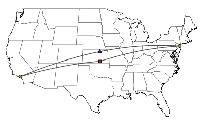The figure to the right shows these two centers along with arcs of great circles connecting them to Los Angeles and New York. Notice that if we were to stand at the point computed using the three-dimensional formula with a very light rod connecting us to Los Angeles and another connecting us to New York, the rods would be of equal length and point in opposite directions. This is what we expect from a balancing point. However, if we stand at the point given by the formulas used by the Census Bureau, the two rods would not point in opposite directions, which means this is not a balancing point.

Notice also that the formulas used by the Census Bureau pull the center of population south from the location determined by the three-dimensional method. This is to be expected for the Census Bureau's method locates the center roughly at the midpoint of a segment drawn between the two cities after the U.S. has been projected onto a map simply using the longitude and latitude. However, in the Northern hemisphere, great circles, the paths of shortest distance on the sphere and therefore the true "straight lines" on the sphere, bend to the north of a line segment in this projection.

If we now consider the figures from the 2000 Census, we see that the Census Bureau locates the center at

$\bar{\phi}=\hbox{37N42},\quad\bar{\lambda}=\hbox{91W34}.$

whereas the three-dimensional method gives

$\hat{\phi}=\hbox{38N47},\quad\hat{\lambda}=\hbox{91W49}$

The Census Bureau's formulas again give a center lying south of that computed by the three-dimensional method by some 78 miles.

Isn't any definition good enough?

Hayford argued that the motion of the center is more important than its location, and consequently the particular method we use for computing the center is not significant as long as we consistently use that method. However, the apparent motion of the center may change considerably when one map projection is chosen over another. It would therefore be most desirable if the center did not depend on any choices, such as that of a map projection, that we make. Furthermore, we would expect that the center of population should depend only on how the population of the U.S. is distributed and not where the U.S. happens to be placed on the Earth. That is, if the U.S. and its population were rotated and shifted down into a more tropical region, we should expect that the center of population is in the same position relative to the rest of the country. This will typically not be the case when we define the center through a choice of map projection.

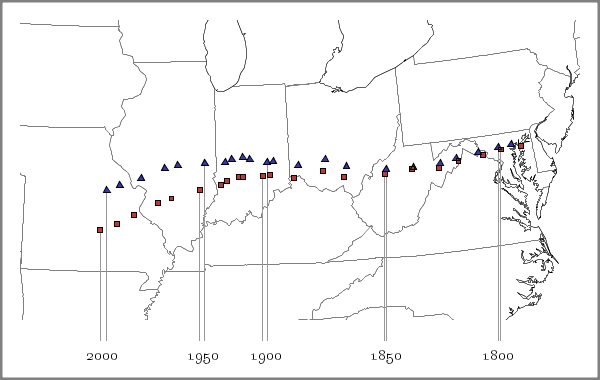
The figure below shows how the two centers--that computed by the Census Bureau () and that computed through our three-dimensional method ()--have moved from the first census in 1790 up to the most recent census in 2000. As expected, both sets of points move to the west. However, the point computed by the Census veers south more quickly than the center computed by the three-dimensional method. When the population was concentrated in a relatively small area, the distortion of distances in a map projection is relatively small and so the difference in the two centers is relatively small. However, as the population has spread out across the continent, the effect of the Earth's curvature has become more pronounced.

A note on the figures

The maps were drawn using the Micro World Data Bank II Database produced and placed in the public domain by Fred Pospechil and Antonio Rivera and based on coordinate data collected by the Central Intelligence Agency. The data is available in the file mwdbpoly.zip. Some of the three-dimensional figures were made using Bill Casselman's ps3d, a PostScript extension for producing three-dimensional mathematical illustrations.

David Austin
Grand Valley State University
david at merganser.math.gvsu.edu

{C}

References

Background

1.	De Jonge, P., The Zip in the Middle, National Geographic, November 2001: 114-21.
2.	A Nation on the Move, National Geographic, May 2002.
3.	O'Connor, J.J. & Robertson, E.F., Herman Hollerith, http://www-groups.dcs.st-and.ac.uk/~history/Mathematicians/Hollerith.html
4.	U.S. Census Bureau, History, http://www.census.gov/acsd/www/history.html, 2003.

Center of Population

5.	Aboufadel, E. & Austin. D., 2004. A new method for computing the center of population of the United States, to appear in The Professional Geographer.
6.	Bachi, R., New methods of geostatistical analysis and graphical presentation. Kluwer, 1999.
7.	Barmore, F.E., Where are we? Comments on the Concept of Center of Population. The Wisconsin Geographer, 9: 8 - 21, 1993. (Reprinted in Solstice: An Electronic Journal of Geography and Mathematics.)
8.	Hayford, J.F., What is the Center of an Area, or the Center of a Population? Publications of the American Statistical Association, 8 (58): 47 - 58, 1902.
9.	U.S. Census Bureau, Census Tracts, http://www.census.gov/geo/www/cob/tr_metadata.html, 2003. Information about census tracts.
10.	U.S. Census Bureau, Centers of Population Computation for 1950, 1960, 1970, 1980, 1990 and 2000. http://www.census.gov/geo/www/cenpop/calculate2k.pdf , 2001. Explains the method used by the Census Bureau to compute the center of population.
11.	U.S. Census Bureau, Centers of Population for Census 2000. http://www.census.gov/geo/www/cenpop/cntpop2k.html, 2002.

Maps

12.	Feeman, T., Portraits of the Earth: A Mathematician Looks at Maps,American Mathematical Society, Providence, 2002.
13.	Snyder, J.P., Map projections: a working manual. U.S. Geological Survey Professional Paper 1395. United States Government Printing Office, 1987.
14.	Map Projections, http://www.colorado.edu/geography/gcraft/notes/mapproj/mapproj_f.html

Curvature and the Theorema Egregium

15.	Gauss, K. F., Disquisitiones generales circa superficies curvas. Dieterich. 1828.
16.	Do Carmo, M., Differential Geometry of Curves and Surfaces, Prentice-Hall, 1976.
17.	O'Neill, B., Elementary Differential Geometry, 273 - 275. Academic, 1966.

Data

18.	U.S. Census Bureau, Population: 1790 to 1990. http://www.census.gov/population/censusdata/table-16.pdf , 1993. Gives the population of the states for each census from 1790 to 2000.
19.	U.S. Census Bureau, Census Tracts, http://www.census.gov/geo/www/cob/tr2000.html, 2003. Cartographic boundary files for the census tracts.
20.	U.S. Census Bureau, Census Tracts, http://www.census.gov/tiger/tms/gazetteer/ustracts2k.txt, 2003. Data from each of the census tracts for Census 2000.