The Mathematics of Rainbows
Posted February 2009.
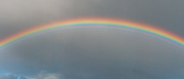
If you look carefully on the inside of the principal violet arc you will frequently see several pale violet arcs, interspersed with some paler greenish bands. Where do they come from?...
Bill Casselman
University of British Columbia, Vancouver, Canada
cass at math.ubc.ca
Introduction
The theory of the rainbow that everyone learns in high school physics classes is pretty much the one that René Descartes came up with almost 400 years ago. But if you look carefully at the rainbow in this picture, just underneath its arch, you will see bands that this familiar theory does not explain.
 |
This remarkable photograph is Double-alaskan-rainbow.jpg from the Wikipedia Commons.
It and all images derived from it in this article are distributed under the Creative Commons Share-Alike license. |
The correct explanation of these bands depends on the wave theory of light developed in the early nineteenth century, primarily by Auguste Fresnel. The correct application of Fresnel's theory to rainbows is due to the English mathematician George Biddell Airy, writing about 1840. This theory was superseded in turn by the electromagnetic theory of Maxwell. The description of the rainbow that Maxwell's theory produces is in some extreme cases quite different from the one produced by the wave theory. But for practical purposes Airy's theory is sufficient.
Airy's theory requires numerical evaluation of an improper integral named after him. How to carry out this evaluation also has an interesting history.
Descartes
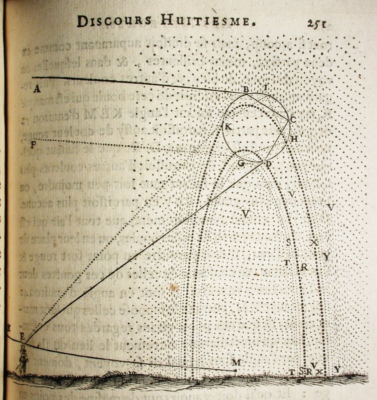
René Descartes, most famous as a philosopher and also as the discoverer (inventor?) of analytic geometry, was responsible for the first detailed study of the rainbow in Europe. This appeared in L'arc en ciel, one of many smaller technical essays concerned with weather and meteorology inserted at the end of his philosophical treatise Discours sur la méthode. This woodcut from the essay, probably made for Descartes by Frans van Schooten the younger, makes things fairly clear (click for a larger image).
In Descartes' scheme, a light ray (here coming from upper left) hits a raindrop, penetrates it, is reflected internally one or more times, and finally exits. When a light ray moves from air to water, it changes direction. We now know - at least in some sense - that this is because the light travels in waves, and it possesses a slower speed inside water. The change in direction is effected according to Snell's Law:
where i is the angle of incidence, r that of refraction, and n is the index of refraction, which is approximately 1.33 for the air/water transition.
The raindrop, assumed to be spherical, is a more complicated surface than a level surface. The ray reflects around inside the drop, maybe several times. The usual rainbow is the result of one reflection, like this:
The total deflection of the ray from its original direction is D = 180+2i-4r, where i is the angle of incidence when the ray first hits the drop and r the refraction angle at first contact.
For a rainbow, all rays come from the same direction, that of the sun. So if we want to understand it, we look at what happens to all the rays hitting the rainbow and coming from a fixed direction. We may as well take this to be infinitely far to the left. Only those rays at height y with |y| ≤ 1 will hit, and for those rays, y = sin i, or i = arcsin y. As Descartes did, we follow a bundle of those rays as they pass through the drop:
What we discover is that the rays bunch up along a certain one of them. This means that there is a great concentration of light in that direction. Since this is what happens also when a magnifying glass concentrates sunlight on paper, it is called the caustic ray.
As the height y of an incoming ray increases from 0 to the radius of the drop, the deflection of the outgoing ray decreases towards that of the caustic ray, and then after y passes the caustic ray the deflection starts to increase again. Here is a graph of deflection plotted against i = arcsin(y):
Descartes apparently found the deflection of the caustic ray by graphical methods. But we have now a better tool - we can find it by solving a minimum problem in calculus. We know that D = 180+2i-4r and r = arcsin(i/n). We calculate dD/di and set it equal to 0. The computation requires remembering that if f(x) = arcsin(x) then f'(x) = 1/√ 1-x2. We get:
dD/di = 2 - 4 (cos i/n)/√(1 - sin2i/n2)
√(1 - sin2i/n2) = 2 cos i / n
1 - sin2i/n2 = 4 cos2 i / n2
1 - 1/n2 = 3 cos2 i / n2
cos i = √ (n2-1)/3 |
which with n=1.33 gives cos i=0.506, i=59.6o.
Newton
Descartes understood roughly why the rainbow is located where it is, but he was fairly straightforward in declaring that he didn't understand why the rainbow showed different colors. In effect, he didn't know that different colors (which we now know to correspond to different wave lengths) of light have different refractive indices n. This was the contribution of Isaac Newton. Here is a table (data taken from Philip Laven's site):
So the caustic rays of different color, all from the same direction, are scattered as they exit the raindrop.
These all go to different observers. To a given observer go caustic rays of different colors, and that's what makes the rainbow.
Airy
Descartes' theory explains the main features of a rainbow quite well - red arc on the outside, violet on the inside, pretty colors in between. But if you look carefully on the inside of the principal violet arc you will frequently see several pale violet arcs, interspersed with some paler greenish bands. These do not occur in Descartes' theory. Where do they come from?
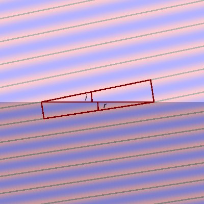
An answer to this question was first supplied by the Cambridge mathematician George Biddell Airy, who applied the wave theory of Fresnel. The wave theory says that the reason for diffraction is that the waves carrying light move forward at slower speed when they cross from air into water. But of course the frequency does not change. We know that
| (wave length) (frequency) = (wave velocity) |
and therefore when they slow down, the wave length decreases. Among other things, this explains Snell's Law, as indicated in this figure:
What happens as wave enters a rain drop is more complicated. Since its surface is curved, the wave front does not remain straight:
What is important in this picture is the way the wave front doubles back on itself, in effect mingling two waves, each with a different front. These two components of the waves mix with each other in a complicated fashion, leading to interference (and those bands of light we are trying to explain). In order to understand what's going on in simple terms, one needs a useful trick - not looking at the true wavefront as it emerges from the drop, but looking instead at a virtual wave front, which is the wave front in clear air that would cause the emerged wave front:
Now we can see that we are in fact looking at a mathematical problem that is quite simple to state (if not to solve) what is the wave propagation from an S shaped wave front?
This is an exercise in Huyghen's principle, which says that a wave can be reconstructed from a single wave front by considering each point on that wave front as an isolated infinitesimal source, all of them contributing to the propagation. If we reorient our coordinate system so that the caustic ray is the negative x-axis, the S-shaped curve may be expressed to a good approximation in the form x = k y3. We may express k = c/R2 where c is a dimensionless constant and R is the radius of the raindrop.
The amplitude of the wave determining light at some far away point in the direction θ is the integral of the contributions at all the points on the cubic curve. According to the figure above, the difference in phase from contributions at (0,0) and (x,y) is (x sin θ - y cos θ)/λ where λ is the wave length concerned. This leads after some calculation to an approximation to the magnitude of the wave at some far away point in direction θ - it is some constant times the infinite integral
where m is proportional to θ. There are a number of simplifications involved here that I am passing along without elaboration - for example, replacing an integral over a finite interval by an infinite one, and approximating sin s by s, and cos s by 1 when s is small.
De Morgan
In order to verify that his theory agreed with phenomena, Airy had to evaluate his integral for various values of m. It seems astonishing to us now to see that the way he did this was by explicit numerical calculation of the integral. Not at all a task undertaken lightly. But then Airy went on to become the Astronomer Royal, best known for the accuracy of the astronomical computations done during his administration rather than flights of imagination. He is in fact most famous for having caused the British mathematician John Couch Adams not to get full credit for predicting the discovery of the planet Neptune. His next moment of fame was his role in engineering design of the great Tay Bridge disaster.
Augustus De Morgan suggested very early in Airy's explorations a way around this tedious procedure, namely an explicit expression for the Taylor series of Airy's integral around m=0.
But Airy refused to use De Morgan's method because De Morgan was unable at first to justify his procedure rigorously, even though his heuristic reasoning seems to have been quite reasonable. De Morgan was finally able to prove the validity of his computations, and in his second article on caustics Airy used the series De Morgan had offered him. Most of this second article, in fact, amounts just to an extract of a letter from De Morgan explaining his argument. De Morgan was well known in his time for other mathematical work, particularly involving Euclid and education, as well as for several popular expositions of mathematics. But his discovery of the calculation of the Taylor series of the Airy integral showed a talent that his work didn't often exhibit.
The series that De Morgan came up was this:
The terms in the series can be calculated easily by recursion. For the first series
t0=1
tn+1 = -tn x3 / 3(3n+2)(3n+3) |
and for the second
t0 = x
tn+1 = -tn x3 / 3(3n+3)(3n+4) . |
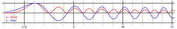
The following figures show the graph of the function, the graph of its square, which is proportional to the magnitude of light, and the resulting "rainbow" for monochromatic light.
Stokes
The Taylor series is useful for small values of m, but for large ones something unpleasant happens. For m large, the terms in the series grow rapidly, but they largely cancel out, leaving very small terms. Because computers handle real numbers with limited precision, the cancellations start to produce more or less random numbers after a while. (This happens already with the far simpler series for ex when x < 0. But there it is no problem, since the series with x > 0 offers no unusual difficulty, and e-x = 1/ex.)) For Airy, this limited the range for which he could compute A(x) to about [-4.0, 5.6].
Airy doesn't seem to have speculated on the obvious pattern the graph was showing, much less how to verify that there might be a way to find a rigorous description of the behavior of A(x) for large values of |x| easing oscillations for x > 0. This challenge was taken up be the Cambridge mathematician George Gabriel Stokes (after whom Stokes' Theorem is named), a man of much greater talent and imagination than Airy, and one of the greatest mathematical physicists of the century. His investigations of Airy's integral led him to some extremely fruitful mathematical ideas.
There were two major contributions by Stokes. The first was that the Airy integral could be approximated for large values of |m| by asymptotic series. The one for m > 0 approximates A(m) by a slowly decreasing oscillation, and the one for m < 0 approximates it by an exponentially decreasing function. These series are expansions in negative powers of m.
First set
Then for m > 0 we have
and for m < 0:
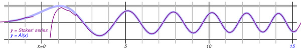
These series do not converge, but the initial terms decrease reasonably rapidly, and the series give fair approximations to A(m) if one breaks off calculation when the terms start to grow. The following compares the exact graph (in light blue) to the ones obtained from Stokes' approximation, following this rule (in violet). After a bumpy start, the approximation looks quite good.
Stokes' first construction of these series was not entirely rigorous. He knew that he had some asymptotic expansions valid in the two regions m > 0 and m < 0, but he could not justify an heuristic rule for getting certain constants correctly. His second contribution was to be able to do this, and in doing so introduce what are now called Stokes lines.
See the continuation of this column, also by Bill Casselman, "The Mathematics of the Rainbow, Part II."
To find out more ...
... about rainbows in general
- C. Boyer, The rainbow: from myth to mathematics, Princeton University Press, 1987.
A reasonably complete if rather dull historical account.
- Jearl Walker, Mysteries of rainbows, notably their rare supernumerary arcs, Amateur Scientist column for Scientific American, June, 1980.
Amateur Scientist, Scientific American July 1977, page 138 - 144: How to create and observe a dozen rainbows in a single drop of water by Jearl Walker. ...
- R. A. R. Tricker, Introduction to meteorological optics, American Elsevier, 1970.
Tricker has written a number of books that are too sophisticated for idiots and too elementary for geniuses. All of them are worth reading. They offer a unique view of interesting aspects of science at an intermediate level. This one is his masterpiece. The chapter on supernumerary bows gives some helpful details on Airy's formula.
- H. Nussenzveig, The theory of the rainbow, Scientific American, April, 1977.
Some idea of the exact theory according to electrodynamics, and modern approximations to it.
- Philip Laven's optics pages
- Les Cowley's web site on atmospheric optics
... about George Biddell Airy
- G. B. Airy, On the intensity of light in the neighborhood of a caustic, Transactions of the Cambridge Philosophical Society VI (1838), 379-403.
- ----------, Supplement to the previous paper, Transactions of the Cambridge Philosophical Society VIII (1849), 595-600.
The Transactions are available from Google books. Search there for "Transactions of the Cambridge Philosophical Society".
- Adams, Airy, and Neptune
Tries to justify Airy's behavior in the incident.
- Wikipedia on the discovery of Neptune
A more standard account.
- Wikipedia entry on Airy
- F. W, J. Olver, Asymptotics and special functions, Academic Press, 1972.
On pages 53-55 you will find the modern version of what De Morgan explained to Airy about finding the Taylor series of the Airy integral. Later in the book you will find the modern version of Stokes' discoveries.
... about George Gabriel Stokes
- G. G. Stokes, On the numerical calculation of a class of definite integrals and infinite series, Transactions of the Cambridge Philosophical Society IX, Part I.
This is the paper in which Stokes proved the validity of the asymptotic expansion of series for Airy's integral, except for one point for which his argument remained heuristic.
- -------, On the discontinuity of arbitrary constants which appear in divergent developments, Transactions of the Cambridge Philosophical Society IX, pp. 106-128.
- ------, Supplement to the previous paper, Transactions of the Cambridge Philosophical Society XI, Part II.
These two papers make rigorous his earlier heuristic argument, introducing into mathematics what we now the Stokes lines (except that some of us call them the anti-Stokes lines).
Bill Casselman
University of British Columbia, Vancouver, Canada
cass at math.ubc.ca
Those who can access JSTOR can find some of the papers mentioned above there. For those with access, the American Mathematical Society's MathSciNet can be used to get additional bibliographic information and reviews of some these materials. Some of the items above can be accessed via the ACM Portal , which also provides bibliographic services.