Welcome to the Feature Column

---

Who's Number 1? Hodge Theory Will Tell Us

This article describes a method, proposed by Jiang, Lim, Yao, and Ye, that uses Hodge theory to rank a large number of alternatives...

Mail to a friend

Print this article

Introduction

Life is full of choices. Particularly in our data-rich world, we are often presented with a wide variety of alternatives from which we would like to choose the best possible. Which website has the best answer to my question, where should I go for lunch, which movie should we watch tonight. Times were simpler when the choice boiled down to John or Paul.

To help make decisions, we often rely on a ranking of the alternatives and choose the ones with the highest rank. For instance, when I search for "Condorcet paradox," Google tells me there are 115,000 results. Like most people, I will most likely rely on Google's ranking and be satisfied with what I find among the top ten.

There is, however, an inherent difficulty in making decisions in which several criteria are condensed into a single ranking. For instance, imagine you have three choices for lunch. The food at Macho Taco is lackluster, but it's cheap, fast, and conveniently located. The food is somewhat better at Chez Fromage and it's affordable and close, but the service is terrible. Meanwhile, Thai One On has good food and service, but it's expensive and far away.

It would not be unreasonable if I preferred

Macho Taco over Chez Fromage,
Chez Fromage over Thai One On, and
Thai One On over Macho Taco.

If we are to have a ranking system, we would expect the rankings to be transitive; that is, if choice A is rated higher than B, and B is rated higher than C, then A is also rated higher than C. However, our lunch preferences are clearly not transitive, a situation known as the Condorcet paradox. This paradox may appear when a single voter compares alternatives based on several factors or when groups of voters are asked to make rankings collectively.

The Condorcet paradox occurs frequently when ranking sports teams. For instance, in the 2010 college football season,

Oklahoma beat Texas Tech, 45 - 6,
Texas Tech beat Missouri, 24 - 17, and
Missouri beat Oklahoma, 36 - 27.

In which order should the three teams be ranked?

This article describes a method, proposed by Jiang, Lim, Yao, and Ye, that uses Hodge theory to rank a large number of alternatives in which the Condorcet paradox may appear. Besides providing a ranking, this method will also create a means of measuring how reliable the ranking is.

The data sets that Jiang et al aim to rank have other complications. Think of restaurant reviews on yelp.com or movies reviewed on Netflix.

• First, the ratings are incomplete; for example, most subscribers will have rated only a small number of movies.
• Second, the ratings are imbalanced; some movies, like summer blockbusters, will have a lot of ratings, while others, like documentaries, will receive only a few.

Finally, humans are not very good at ranking large numbers of alternatives. In a seminal paper in cognitive psychology, George Miller demonstrated that we have a hard time evaluating more than seven options. This may be why yelp and Netflix only allow us five stars.

Comments?

Pairwise comparison graphs

To construct a ranking, we build a pairwise comparison graph $G$ as follows. Suppose that we have a set of objects $V=\{1,2,\ldots,n\}$ to be ranked and a set of voters, each of whom has compared pairs of objects and expressed a preference for one object in each pair.

Examples include:

• The set $V$ of web pages. The voters are also considered to be the set of web pages, which express a preference for other pages by linking to them. This is the heart of Google's PageRank algorithm.
• The set $V$ of movies in the Netflix movie library. Voters are subscribers who have rated movies on a scale of one to five stars.
• The set $V$ of college football teams. The voters are games played between teams, with a preference expressed for the winner of the game.

Sometimes, preferences between pairs may be inferred from other rating data. For instance, if a voter has rated movie $i$ in the Netflix movie database with four stars and movie $j$ with two stars, we may infer a preference for movie $i$ over $j$.

We define $w^\alpha_{ij} = 1$ if voter $\alpha$ has made a comparison between item $i$ and $j$, and $w^\alpha_{ij} = 0$ if not. The number of voters who have compared $i$ and $j$ is $w_{ij}=\sum_\alpha w^\alpha_{ij}$.

In the pairwise comparison graph $G$, the set of objects $V$ to be ranked forms the vertex set. An (undirected) edge joins items $i$ and $j$ if at least one voter has compared $i$ and $j$, that is, if $w_{ij}> 0$. The set of edges will be denoted by $E$, and individual edges will be denoted by a set of vertices, such as $\{i,j\}\in E$.

To each voter $\alpha$ is associated a matrix $Y^\alpha_{ij}$ measuring that voter's "degree of preference" for alternative $i$ over $j$. The degree to which $i$ is preferred over $j$ will be minus the amount that $j$ is preferred over $i$. In other words, $Y^\alpha_{ij} = -Y^\alpha_{ji}$. If voter $\alpha$ has not compared $i$ and $j$, then $Y^\alpha_{ij} = 0$. In any case, since for all $i$ and $j$, $Y^\alpha_{ij} = -Y^\alpha_{ji}$, $Y^\alpha$ is called a skew-symmetric matrix.

The preferences of individual voters are aggregated into a single preference matrix $Y_{ij}$ by, perhaps, averaging the preferences of all the voters who have compared $i$ and $j$. In this case, $Y$ is also skew-symmetric.

The matrix $Y$ belongs to the vector space $C^1$ of all skew-symmetric $n\times n$ matrices $X$ where $X_{ij} = 0$ if $\{i,j\}$ is not an edge of $G$. Such a matrix will be called an edge flow, terminology that calls attention to its interpretation as the flow of "preference" along an edge from higher to lower preference. Preference will flow out of vertices with a higher ranking and into vertices with a lower ranking. In this way, we may imagine a motivating comparison between edge flows and vector fields on, say, ${\Bbb R}^3$ that describe the flow of a gas from an area of high pressure to one of low pressure.

In search of a potential

Armed with our pairwise comparison graph, we would like to find a ranking of the objects $V$ that is compatible with the pairwise comparisons. In particular, we would like to assign to each object $i$ a ranking $s_i$ such that $Y_{ij} = s_i-s_j$ if a comparison has been made between $i$ and $j$. In other words, the ranks of two objects should differ by the amount that one is preferred over the other.

Let's put this into a larger framework and define the vector space $C^0$ to be ${\Bbb R}^n$, which we think of as the set of functions on $V$. We may define the gradient as a map

 

\[{\rm grad}:C^0 \longrightarrow C^1\]

by \[{\rm grad} (s)_{ij} = s_j-s_i.\]

Given our preference matrix $Y$, our desired ranking function will be a potential $s$ such that $Y = -{\rm grad}(s)$.

Consideration of the Condorcet paradox shows that a potential function is not guaranteed, or even likely, to exist. Remember that the Condorcet paradox says that it is possible to prefer $i$ to $j$, $j$ to $k$, and $k$ to $i$. In other words, we could have

 

\[Y_{ij} + Y_{jk} + Y_{ki} > 0.\]

However, if $Y=-{\rm grad}(s)$, then

 

\[Y_{ij} + Y_{jk} + Y_{ki} = (s_i-s_j) + (s_j-s_k)+(s_k-s_i) = 0.\]

For this reason, we need to consider the set of triangles $T$ on the graph $G$. A triangle is a subset $\{i,j,k\}$ of $V$ where $\{i,j\}$, $\{j,k\}$, and $\{k,i\}$ are edges of $G$. We also introduce the vector space $C^2$ of hypermatrices $\Phi_{ijk}$, where $\{i,j,k\}$ is a triangle, along with the symmetry condition

 

\[\Phi_{ijk} = \Phi_{jki} = \Phi_{kij} = -\Phi_{jik} = -\Phi_{ikj} = \Phi_{kji},\]

We may now define the function ${\rm curl}:C^1\longrightarrow C^2$ by

 

\[{\rm curl}(X)_{ijk} = X_{ij}+X_{jk} + X_{ki}.\]

Using our preference edge flow $Y$, a triangle with ${\rm curl}(Y)_{ijk} \neq 0$ is called a triangular inconsistency because the voters' preferences are not transitive along that triangle.

Putting everything together, we have

 

\[ C^0 \stackrel{{\rm grad}}{\longrightarrow} C^1 \stackrel{{\rm curl}}{\longrightarrow} C^2 \]

and ${\rm curl}({\rm grad}(s)) = 0$.

At this point, there is a lot of notation so let's briefly summarize where we are. Individual voters' preferences are aggregated into an edge flow $Y\in C^1$. We are seeking a ranking of the objects in $V$, which will be given by a potential function $s \in C^0$, where $Y=-{\rm grad}(s)$. If a potential function exists, our preference edge flow must satisfy ${\rm curl}(Y) = 0$.

Comments?

The Hodge decomposition

Hodge theory gives us a useful decomposition of $C^1$. First, we will consider ${\cal G}$, which is the image of ${\rm grad}$ in $C^1$. That is, ${\cal G} = {\rm im}({\rm grad})$ meaning that ${\cal G}$ consists of all edge flows $X$ where $X={\rm grad}(s)$ for some potential $s$.

The preference edge flow $Y$ given by aggregating voters' preferences is in $C^1$. If a ranking $s$ exists, then $Y=-{\rm grad}(s)$ should lie in ${\cal G}\subset C^1$. The Condorcet paradox, however, indicates that this may not happen. Instead, we seek a ranking function $s$ such that $-{\rm grad}(s)$ is the closest possible to $Y$.

To measure distances in $C^1$, we need to introduce an inner product. For edge flows $X, Y \in C^1$, we define:

 

\[ \langle X, Y\rangle = \sum_{\{i,j\}\in E} w_{ij}X_{ij}Y_{ij}.\]

Using this inner product, we will see that $C^1$ admits an orthogonal decomposition, known as the Hodge decomposition.

 

\[ C^1 = {\cal G} \oplus {\cal H} \oplus {\cal I}.\]

This decomposition is rather elementary and is demonstrated by a couple of points, including the determination of ${\cal G}$, ${\cal H}$, and ${\cal I}$, that we will bullet below.

 

• Recall that if $f:V\to W$ is a linear map between inner product spaces, then there is an adjoint map $f^*:W\to V$ defined by $\langle f(v), w\rangle = \langle v, f^*(w)\rangle$.

  The image of $f$ is the orthogonal complement of the kernel of $f^*$, the vectors $w$ where $f^*(w)=0$; that is, ${\rm im}(f) = {\rm ker}(f^*)^\perp$. This is implied by the equation $\langle f(v), w\rangle = \langle v, f^*(w)\rangle=0$.

• We will introduce inner products on $C^0$ and $C^2$ so that

   

  • If $r, s\in C^0$, then

     

    \[ \langle r, s\rangle = \sum_{i\in V} r_is_i.\]
  • If $\Phi, \Psi\in C^2$, then

     

    \[ \langle \Phi, \Psi\rangle = \sum_{\{i,j,k\}\in T} \Phi_{ijk}\Psi_{ijk}.\]
• The gradient is a linear map ${\rm grad}:C^0\to C^1$ so its adjoint ${\rm grad}^*:C^1\to C^0$ is defined by $\langle {\rm grad}(s), X\rangle = \langle s, {\rm grad}^*(X)\rangle$. This adjoint ${\rm grad}^*$ is more familiarly known as the divergence, and a simple computation shows that

   

  \[{\rm div}(X)_i={\rm grad}^*(X)_i = \sum_{\{i,j\}\in E} w_{ij}X_{ij}.\]

  Similarly, the curl is a map ${\rm curl}:C^1\to C^2$, which gives its adjoint ${\rm curl}^*:C^2\to C^1$ by $\langle {\rm curl}(X), \Phi\rangle = \langle X, {\rm curl}^*(\Phi)\rangle$.

• Remember that ${\cal G} = {\rm im}({\rm grad})$ so we have the orthogonal decomposition

   

  \[C^1 = {\cal G} \oplus {\cal G}^\perp\] where ${\cal G}^\perp = {\rm im}({\rm grad})^\perp = {\rm ker}({\rm grad}^*)$.
• We will define another subspace of $C^1$ to be ${\cal I} = {\rm im}({\rm curl}^*)$. Notice that ${\cal I}^\perp = {\rm ker}({\rm curl})$.

  Since we have ${\rm curl}\circ{\rm grad} = 0$, it follows that ${\rm grad}^*\circ{\rm curl}^* = 0$. In other words, ${\cal I} = {\rm im}({\rm curl}^*) \subset {\rm ker}({\rm grad}^*) = {\cal G}^\perp$.

  We therefore arrive at the Hodge decomposition:

   

  \[C^1 = {\cal G}\oplus{\cal H} \oplus{\cal I}\]

  where

  ${\cal G} = {\rm im}({\rm grad})$,
  ${\cal I} = {\rm im}({\rm curl}^*)$, and
  ${\cal H} = {\cal G}^\perp\cap{\cal I}^\perp = {\rm ker}({\rm div}) \cap {\rm ker}({\rm curl})$.

  The edge flows in ${\cal H}$ are sometimes called harmonic.

Comments?

Applying the Hodge decompostion to rankings

How does this help us to develop a ranking from our preference edge flow $Y$? Since $Y\in C^1$, we may decompose $Y$ as

 

\[Y = -{\rm grad}(s) \oplus H \oplus {\rm curl}^*(\Phi)\]

where the three terms have the following significance:

• $s$ is the potential with the minimal distance between $Y$ and $-{\rm grad}(s)$. As such, this is the best potential for ranking the objects in $V$.

• $\parallel Y - (-{\rm grad}(s))\parallel = \parallel h\oplus {\rm curl}^*(\Phi)\parallel$ measures the distance between $Y$ and the gradient of our ranking. It is therefore a measure of how reliable $s$ is as a ranking.

• Since $H \in {\cal H} \subset {\rm ker}({\rm curl})$, it admits no triangle inconsistencies; that is, $H_{ij} + H_{jk} + H_{ki} = 0$. However, $H$ may contain inconsistencies over longer circuits in $G$; that is, $H_{i_0i_1} + H_{i_1i_2} + H_{i_2i_3} + \ldots + H_{i_ni_0} \neq 0$. We therefore think of $H$ as describing the global inconsistencies in the preferences $Y$. If $\parallel H \parallel$ is large, this indicates that the ranking is not reliable on a global scale.

• Notice that ${\rm curl}(Y) = {\rm curl}({\rm curl}^*(\Phi))$ meaning ${\rm curl}^*(\Phi)$ contains all the information about local inconsistencies in the ranking. If $\parallel {\rm curl}^*(\Phi)\parallel$ is large and $\parallel H\parallel$ small, the ranking is reliable on a global scale, but perhaps not on a smaller scale. For instance, if we are ranking 100 objects, it may not be reasonable to think that object 30 is preferred to 31 and 31 preferred to 32. However, it would be reasonable to conclude that object 5 is preferred to object 30.

Computing the decomposition

We will now describe a simple method for computing the decomposition of the preference edge flow $Y$, beginning with the computation of $s$.

We seek the potential that minimizes $\parallel Y-(-{\rm grad}(s))\parallel^2=\parallel Y+{\rm grad}(s)\parallel^2$ among all $s\in C^0$. Therefore, if $r$ is any other potential,

 

\[ \begin{array}{rcl} \frac{d}{dt} \parallel Y+{\rm grad}(s+tr)\parallel^2\mid_{t=0} &=& \frac{d}{dt} \langle Y+{\rm grad}(s+tr), Y+{\rm grad}(s+tr)\rangle\mid_{t=0} \\ & = & 2\langle{\rm grad}(r), Y+{\rm grad}(s) \rangle\\ & = & 2\langle r, {\rm grad}^*(Y+{\rm grad}(s)) \rangle \\ & = & 0, \end{array} \]

which implies that

 

\[{\rm grad}^*\circ {\rm grad}(s) = -{\rm grad}^*(Y).\]

This is known as the normal equation that arises in the solution of a least-squares problem, and there are standard techniques for solving it. The map ${\rm grad}^*\circ {\rm grad}$ is sometimes called the Helmholtzian and denoted $\Delta_0$. The normal equation in this form is:

 

\[\Delta_0 s = -{\rm div} \thinspace Y.\]

In the same way, we may find $\Phi$ by minimizing $\parallel Y-{\rm curl}^*(\Phi)\parallel^2$. This leads to the normal equation

 

\[{\rm curl}\circ {\rm curl}^*(\Phi) = {\rm curl}(Y),\]

which may also be solved with standard techniques.

Comments?

The BCS college football standings

When reading Jiang et al's paper, I wanted to find a data set that I could use to explore the ideas computationally. There are plenty of places where these ideas apply, and Jiang et al describe several.

Wanting a relatively small data set that I could analyze quickly on my laptop, however, I chose to look at the 2010 college football season. Besides, as The New York Times recently pointed out, any yokel with a computer has a college football ranking system, and, well, I have a computer.

Under my system, the objects $V$ to be ranked are the 120 Division I college football teams. The voters are games between two Division I teams, which create pairwise comparisons.

There are many ways in which games could be used to create a comparison between teams. In computer rankings used in the BCS (Bowl Championship Series) standings, however, the NCAA does not allow the margin of victory to be used. Therefore, I used a simple comparison, where $Y^\alpha_{ij} = 1$ if team $i$ beat team $j$ in game $\alpha$. I also experimented with other possibilities that included the margin of victory, which sometimes had significant effects on the rankings.

This seems like an appropriate, though perhaps not ideal, application of our Hodge theoretic ideas. Here are some facts about the comparison graph $G$.

• There were 683 regular games played between Division I teams. I am including conference championship games in the regular season, since they are used in determining the BCS rankings, which determine the bowl game matchups.

• There were 965 triangles formed by sets of three teams, each of whom has played the others. Since $Y_{ij} = \pm 1$, the curl of $Y$ around any triangle will be either $\pm1$ or $\pm3$. In other words, every triangle demonstrates a triangular inconsistency. However, the triangles whose curl is $\pm3$ represent the ones in which team A beat team B, which beat team C, which beat team A. There were 122 triangles, out of the 965, that demonstrated such inconsistencies.

• The data is incomplete. Generally speaking, each of the 120 teams plays about 12 games. Therefore, most pairs of teams will not be compared. College football differs from professional football in that there are many teams, most of whom do not play one another.

• The data is balanced. Each team has roughly the same number of comparisons since each team plays about 12 games.

• There is little need for aggregating comparisons since most pairs of teams play at most one game. There were, however, two pairs of teams that played twice during the regular season. In other words, $w_{ij} = 0$ or $1$ most frequently.

  It would be possible, however, to include different voters in this system, by considering other statistics from the games, such as total offense or whether the winning team was the home or away team. I have not done this, however.

At the end of the regular season, college football teams are ranked according to the BCS standings, which combine a number of computer ranking systems along with polls of sportswriters and football coaches. Based on these rankings, the top two teams advance to a national championship game, the winner of which is declared to be the national champion.

The 2010 season was somewhat controversial since, when the regular season ended, three teams---Auburn, Oregon, and Texas Christian---were undefeated yet only two could advance to the national championship game. The final BCS standings, announced on December 5, 2010, the day after the regular season ended, had Auburn and Oregon in the top two positions, much to the displeasure of Texas Christian fans.

Shown below is a comparison of the BCS ranking and our Hodge-theoretic ranking, as of December 5, 2010. I have normalized the Hodge theoretic rankings so that the highest ranked team has a score of 100 and the lowest ranked team has 0.

 

	BCS Ranking	Hodge Theoretic Ranking
1	Auburn (13-0), 0.9742	Auburn, 100.0
2	Oregon (12-0), 0.9831	Oregon, 97.7
3	TCU (12-0), 0.9139	Oklahoma, 94.2
4	Stanford (11-1), 0.8400	Stanford, 92.9
5	Wisconsin (11-1), 0.8651	Missouri, 91.3
6	Ohio State (11-1), 0.8046	Texas Christian, 91.2
7	Oklahoma (11-2), 0.6758	Arkansas, 89.0
8	Arkansas (10-2), 0.6989	Louisiana State, 87.9
9	Michigan State (11-1), 0.7382	Texas A&M, 86.8
10	Boise State (11-1), .6316	Oklahoma State, 85.3

Interestingly, the Hodge-theoretic ranking promoted Oklahoma, a team with two losses to highly-ranked Missouri and Texas A&M, over Texas Christian, a team with no losses. This has nothing to do with this author growing up in a family of die-hard Oklahoma fans. Rather, the effect of the two losses is mitigated by their appearance in three triangles in which $A$ beat $B$ who beat $C$ who beat $A$.

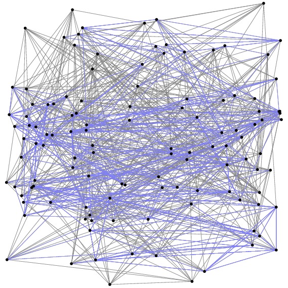
The figure below shows the pairwise comparison graph $G$. Edges are shown in gray, and triangles in which $A$ beat $B$ beat $C$ beat $A$ are in blue. The height of vertex $i$ in the figure is equal to $s_i$.

 

For the sake of completeness, I feel compelled to report that lowly Akron earned the minimal score of 0.0, thereby justifying their team name, the Zips.

Of course, the Hodge-theoretic approach gives us more than just the ranking since we have a decomposition of the preference edge flow $Y$ as

 

\[Y=-{\rm grad}(s) \oplus H \oplus {\rm curl}^*(\Phi).\]

For the data set above, I computed

 

\[\parallel Y \parallel = 26.13,\quad \parallel -{\rm grad}(s) \parallel = 18.17,\quad \parallel H \parallel = 8.17,\quad \parallel {\rm curl}^*(\Phi) \parallel = 16.9.\]

Remember that $H$ is a measure of the global inconsistencies in $Y$. It is unreasonable to expect $H$ to be too small since there will certainly be long loops of inconsistencies. Still, its size is modest compared to the gradient term so we may have some degree of confidence in our ranking.

Also, ${\rm curl}^*(\Phi)$ measures the triangular inconsistencies. Since every triangle is inconsistent due to the fact that $Y_{ij}=\pm1$, we should expect this component to be significant.

After the bowl games were played, the final rankings look like this:

 

	Associated Press Poll	Hodge Theoretic Ranking
1	Auburn	Auburn, 100.0
2	Texas Christian	Stanford, 94.0
3	Oregon	Oregon, 93.3
4	Stanford	Texas Christian, 91.0
5	Ohio State	Oklahoma, 89.1
6	Oklahoma	Louisiana State, 89.0
7	Wisconsin	Boise State, 83.2
8	Louisiana State	Alabama, 83.0
9	Boise State	Arkansas, 82.6
10	Alabama	Ohio State, 82.5

Comments?

Summary

Readers familiar with vector calculus will no doubt be struck by the use of the terms gradient, curl, and divergence, which originate in a study of functions and vector fields in Euclidean space. In fact, Hodge theory was originally developed in this context as a means of measuring global topological features of Euclidean-like spaces. It has found important and varied applications in topology, algebraic geometry, electricity and magnetism, and a range of other disciplines.

The novel contribution of Jiang et al's paper is to recognize how the Hodge decomposition applies in this combinatorial setting to create rankings and a measurement of their reliability in cases where the data set is incomplete and imbalanced.

Careful readers will have noticed that our ranking depends on several choices. In the specific example I looked at, $Y_{ij}$ is a measurement of the quality of a victory in a football game, and there is an endless variety of ways to perform this measurement. In other situations that require aggregating many voters' preferences, there are also several options that should be considered. Finally, the Hodge decomposition depends on the choice of an inner product on the spaces $C^0$, $C^1$, and $C^2$. There are clearly other choices, which will lead to different rankings.

Rankings have been the inspiration for a great deal of mathematical investigation and are related to important problems in voting theory and social choice, more generally. I have not attempted to place these ideas in the context of this literature. However, in their extremely readable paper, Jiang and his co-authors describe how the Hodge theoretic ranking, along with suitable choices for the inner products, generalize more widely known constructions, such as the Borda count and Kemeny optimal ranking.

Thanks

Thanks to my west Michigan sports authority Trevor "T-Dime" Deimel for help in thinking about how to measure the quality of a football win.

References

• Xiaoye Jiang, Lek-Heng Lim, Yuan Yao, and Yinyu Ye. Statistical ranking and combinatorial Hodge theory, Mathematical Programming, Series B, Vol. 127 (1), 203-244, 2010.

  Available at http://www.stanford.edu/~yyye/hodgeRank2011.pdf

  This paper is very well written. The introduction provides a much more expansive description of the broader subject than I have been able to include here.

• Wikipedia's page on the Condorcet paradox.
   
• George A. Miller. The Magical Number Seven, Plus or Minus Two: Some Limits on our Capacity for Processing Information, Psychological Review, Vol. 63, 81-97, 1956.

  A foundational paper in cognitive psychology.

• Jonathan Hodge. The Mathematics of Voting and Elections: A Hands-On Approach. American Mathematical Society, 2005.

  This undergraduate text gives a compelling introduction to a number of important mathematical issues in voting theory and social choice. This Hodge is not related to the Hodge of Hodge theory leaving us with something of a hodge-podge.