Feeling Your Way Around in High Dimensions
The simplest objects of interest in any dimension, which are also the basis for approximating arbitrary objects, are the convex polytopes and in this column I'll explain how to begin to probe them...
 Bill Casselman
University of British Columbia, Vancouver, Canada
Email Bill Casselman
Introduction
Visualization of objects in dimensions greater than three is not possible, which means that it is very difficult to comprehend objects in those dimensions. You cannot see the whole thing all in one glance. All one can do is probe with mathematics to verify a limited number of selected properties, like the proverbial blind men dealing with the elephant. The simplest objects of interest in any dimension, which are also the basis for approximating arbitrary objects, are the convex polytopes and in this column I'll explain how to begin to probe them.
Convex polytopes occur in many applications of mathematics, particularly related to linear optimization problems in the domain of linear programming. There is a huge literature on this topic, but I shall be interested in something different, because even in theoretical mathematics interesting problems involving convex polytopes arise. The terminology traditionally used in linear programming originated in applications, perhaps with non-mathematicians in mind, and it diverges considerably from standard mathematical terminology. Instead, I shall use notation more conventionally used in geometry.
What is a convex polytope?
In any dimension $n$, a convex set is one with the property that the line segment between any two points in it is also in the set. For example, billiard balls and cubes are convex, but coffee cups and doughnuts are not. There is another way to characterize convex sets, at least if they are closed: A closed convex set is the intersection of all closed half planes containing it.

There is a third way to characterize closed convex sets. The convex hull of any subset $\Sigma$ of ${\Bbb R}^{n}$ is the set of all linear combinations $$ \sum_{i=1}^{m} c_{i} P_{i} $$ with each $P_{i}$ in $\Sigma$, each $c_{i} \ge 0$, and $\sum c_{i} = 1$. If the set has just two elements in it, this is the line segment between them, and if it has three this will be the triangle with these points as vertices. In general, each point of the convex hull of $\Sigma$ is a weighted average of points in $\Sigma$. A point of a set is extremal if it is not in the interior of a line segment between two points of the set. For example, the points on the unit sphere are the extremal points of the solid sphere, and the extremal points of a cube are its corners. Every closed convex set is the convex hull of its extremal points.
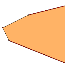
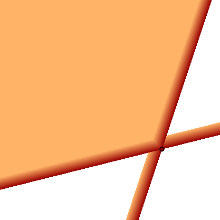
A closed convex set is called a polytope if it is the convex hull of a finite number of points and rays, like this:
Any closed convex set is the intersection of a collection of half-planes, but for a polytope this collection may be taken to be finite. In other words, a convex polytope is the intersection of a finite number of half-spaces $f(x) \ge 0$, where $f$ is a function defined by a formula $$ f(x) = \Big(\sum_{i=1}^{n} c_{i} x_{i}\Big) + c_{n+1}. $$
So there are two ways in which a polytope might be handed to you, so to speak. In the first, you are given a finite set of points and a finite set of rays, and the polytope is the convex hull of these. In the other, you are given a finite collection of affine functions $f_{i}(x)$, and the polytope is the intersection of the regions $f_{i}(x) \ge 0$. Each of these two ways of specifying a polytope is important in some circumstances, and one of the basic operations in working with convex polytopes is to transfer back and forth between one specification and the other.
There are other natural questions to ask, too. A face of a polytope is any one of the polytopes on its boundary. A facet is a proper face of maximal dimension. Here are some natural problems concerning a given convex polytope, which I suppose given as the intersection of half-planes:
-
to tell whether the region is bounded;
-
if it is bounded, to find its extremal vertices, and if not, its extremal edges as well;
-
if it is bounded, to find its volume;
-
to find the maximum value of a linear function on the polytope;
-
to find the dimension of the polytope (taken to be $-1$ if the region is empty, which it may very well be).
But here I have space for exactly one of these questions and some related issues: How to find the dimension of a polytope specified by a set of inequalities? This is by no means a trivial matter. For example, the inequalities
|
$$ \eqalign { x &\ge 0 \cr y &\ge 0 \cr x + y &\le 1 \cr } $$ |
 |
define a triangle, whereas
|
$$ \eqalign { x &\ge 0 \cr y &\ge 0 \cr x + y &\le 0 \cr } $$ |
 |
specifies just the origin, and
|
$$ \eqalign { x &\ge 0 \cr y &\ge 0 \cr x + y &\le -1 \cr } $$ |
 |
specifies an empty set. So the answer to the question does not depend on just the algebraic form of the inequalities.
I include also links to a collection of Python programs that illustrate what I say in a practical fashion.
Comments?
Affine functions and affine transformations
The basic idea of of dealing with a convex polytope is to find one or more coordinate systems well adapted to it. I shall assume that the inequalities you are given to start with are all of the form $f(x) \ge 0$, where $f(x)$ is an affine function, one of the form $\Big(\sum_{i=1}^{n} c_{n}x_{n}\Big) + c_{n+1}$. This differs from a linear function by the presence of the constant. This assumption is easy enough to arrange by changing signs and shifting variables from one side of an equation to another.
A coordinate system well adapted to a polytope will have as origin a vertex of the polytope. But there is one technical point to be dealt with, right off. There might not be any vertices!. There are two possible reasons for this. One is that the region defined by the inequalities might be empty. But there is another possibility. The region $x + y - 1 \ge 0$ in ${\Bbb R}^{2}$ has no vertices--every point in it is in a line segment between two other points in the region. A similar example, although not so evidently, is the region $\Omega$ defined by the inequalities $$ \eqalign { x + y + z + 1 &\ge 0 \cr x &\ge 0 \cr y + z - 2 &\ge 0 \cr } $$ in 3D. Seeing this requires a small amount of work. The point is that the linear parts of the group of functions here are linearly dependent, since $$ x+ y + z = x + (y+z) $$ The planes $x=0$ and $y+z=0$ intersect in a line through the origin, which happens to be the line through the vector $[0, 1, -1]$. The functions $x$ and $y+z$, hence also $x+y+z$ are invariant along lines parallel to this line. If $P$ is any point in $\Omega$, so are all the points $P + t[0, 1, -1]$. Another way of saying this is that the functions defining $\Omega$ are all invariant with respect to translations by scalar multiples of the vector $[0, 1, -1]$.
This suggests that to understand any region $\Omega$ defined by inequalities $f_{i}(x) \ge 0$, we must find out all the vectors whose translations leave the functions $f_{i}(x)$ invariant. Once we know that, we shall reduce the complexity of our problem by looking at a slice through the region that is not invariant under any of these, and which does have vertices. We may as well take this to be $\Omega$ in subsequent probing.
We shall do this at the same time we carry out another simple but necessary task. The inequalities defining $\Omega$ have no particular relationship to whatever coordinate system we start with. We would like to find a coordinate system that is somehow adapted to it. A first step is to require:
I. The coordinates are among the affine functions specifying $\Omega$ to start with.
A second step is to require:
II. The origin of the coordinate system must be a vertex of $\Omega$.
I'll call a coordinate system satisfying both conditions a coordinate system adapted to $\Omega$ at that vertex. Having such a coordinate system is equivalent to being given a linear basis of unit vectors at that point, which I'll call a vertex frame. In a first phase of computation we shall find a coordinate system satisfying I, and find one satisfying II in a second phase. In satisfying I, we shall compute at the same time the translations leaving the original $\Omega$ invariant.
So, given the original inequalities, we are going to make some coordinate changes, first to get I, then to get both I and II. These will be affine coordinate changes. The way to do this is hinted at by the example we have already looked at. If we take as new coordinates the functions $$ X = x, Y = y+z-2, Z = z $$ the inequalities can be expressed as $$ \eqalign { X &\ge 0 \cr Y &\ge 0 \cr X + Y - 1 &\ge 0 \, . \cr } $$
From these equations we can see that the region is invariant with respect to translations along the $Z$-axis (in the new coordinates), and that the new origin $(X, Y) = (0, 0)$ is a vertex of the slice $Z = 0$ of $\Omega$.
Comments?
Affine coordinate changes
Suppose we start with coordinates $(x_{1}, x_{2})$ in two dimensions. An affine coordinate change to new coordinates $(y_{1}, y_{2})$ is determined by a pair of equations $$ \eqalign { x_{1} &= a_{1,1}y_{1} + a_{1,2}y_{2} + a_{1} \cr x_{2} &= a_{2,1}y_{1} + a_{2,2}y_{2} + a_{2} \cr } $$ or, more succinctly, as a single matrix equation $$ \left[ \matrix { x_{1} \cr x_{2} \cr } \right ] = \left[ \matrix { a_{1,1} & a_{1,2} \cr a_{21,} & a_{2,2} \cr } \right ] \left[ \matrix { y_{1} \cr y_{2} \cr } \right ] + \left[ \matrix { a_{1} \cr a_{2} \cr } \right ] \quad {\rm or} \quad x = Ay + a \, . $$ There is another useful way to write this, too: $$ \left [ \matrix { x \cr 1 \cr } \right ] = \left[ \matrix { A & a \cr 0 & 1 } \right ] \left [ \matrix { y \cr 1 \cr } \right ] $$ The matrix $\left[ \matrix { A & a \cr 0 & 1 } \right ]$ is called an affine transformation matrix.
If we are given an affine function $f(x) = c_{1}x_{1} + c_{2}x_{2} + c$, what is its expression in the new coordinates? We can figure this out by doing only a small amount of calculation. The expression for $f$ can be written as a matrix equation, since $$ c_{1}x_{1} + c_{2}x_{2} + c = \left [ \matrix { c_{1} & c_{2} & c } \right ] \left [ \matrix { x_{1} \cr x_{2} \cr 1 } \right ] $$ But if we change coordinates from $x$ to $y$ we have $$ f(x) = \left [ \matrix { c_{1} & c_{2} & c } \right ] \left [ \matrix { x \cr 1 \cr } \right ] = \left [ \matrix { c_{1} & c_{2} & c } \right ] \left[ \matrix { A & a \cr 0 & 1 } \right ] \left [ \matrix { y \cr 1 \cr } \right ] $$ so the vector of coefficients of $f$ in the new system is $$ \left [ \matrix { c_{1} & c_{2} & c } \right ] \left[ \matrix { A & a \cr 0 & 1 } \right ] \, . $$ More tediously: $$ \eqalign { f &= c_{1}x_{1} + c_{2}x_{2} + c \cr &= c_{1}(a_{1,1}y_{1} + a_{1,2}y_{2} + a_{1}) + c_{2}(a_{2,1}y_{1} + a_{2,2}y_{2} + a_{2} ) + c \cr &= (c_{1}a_{1,1} + c_{2}a_{2,1}) y_{1} + (c_{1}a_{1,2} + c_{2}a_{2,2}) y_{2} + (c_{1}a_{1} + c_{2}a_{2} + c) \, . \cr } $$ Theorem. If we are given an array of row vectors defining affine functions $$ F_{x} = \left[ \matrix { f_{1} \cr f_{2} \cr \dots \cr f_{M} \cr } \right ] $$ then applying an affine coordinate transformation will change it to the array whose rows are now given in new coordinates $$ F_{y} = F_{x} \left[ \matrix { A & a \cr 0 & 1 \cr } \right ] \, . $$
Finding a good affine basis
How do we find a coordinate system satifying condition I? Let's re-examine an earlier example. In slightly different notation, we started with the matrix of affine functions $$ F_{x} = \left [ \matrix { 1 & 1 & 1 & \phantom{-}1 \cr 1 & 0 & 0 & \phantom{-}0 \cr 1 & 1 & 0 & -2 \cr } \right ] $$ We happened to notice, essentially by accident, that by a change of variables this became $$ F_{y} = \left [ \matrix { 1 & 0 & 0 & 0 \cr 0 & 1 & 0 & 0 \cr 1 & 1 & 0 & 1 \cr } \right ] $$ How exactly do we interpret this? How can we do this sort of thing systematically?
The rows of the new matrix still represent the original affine functions, but in a different coordinate system. In this new coordinate system, a subset of the rows will hold a version of the identity matrix. In this example, it is a copy of $I_{2} = \left[\matrix { 1 & 0 \cr 0 & 1 \cr } \right ]$. The corresponding affine functions are a subset of the new coordinates. Ideally, we would get a copy of the full identity matrix $I_{3}$, but in this case the inequalities are in some sense degenerate, and this matches with the related facts (1) we get $I_{2}$ rather than $I_{3}$ and (2) the third column of the new matrix is all zeroes. Very generally, if we start with $m$ inequalities in $n$ dimensions, corresponding to an $m \times (n+1)$ matrix, we want to obtain another $m \times (n+1)$ matrix some of whose rows amount to some $I_{r}$, with $n-r$ vanishing columns. In this case, the inequalities will be invariant with respect to translations by a linear subspace of dimension $n-r$, and in order to go further we want to replace the original region by one in dimension $r$. We do this by simply eliminating those vanishing columns.
How do we accomplish this? By the familiar process of Gaussian elimination applying elementary column operations. In doing this, we shall arrive at something that looks first like $$ \left [ \matrix { 1 & 0 & 0 & 0 & * \cr 0 & 1 & 0 & 0 & * \cr * & * & 0 & 0 & * \cr 0 & 0 & 1 & 0 & * \cr * & * & * & 0 & * \cr * & * & * & 0 & * \cr * & * & * & 0 & * \cr } \right ] \; , $$ and then upon reduction to a slice $$ \left [ \matrix { \, 1 & 0 & 0 & * \cr 0 & 1 & 0 & * \cr * & * & 0 & * \cr 0 & 0 & 1 & * \cr * & * & * & * \cr * & * & * & * \cr * & * & * & * \cr } \right ] \; . $$ If the rows giving rise to $I_{r}$ are the $f_{i}$ with $i$ in $I$, then they form the basis of the new coordinate system. In this example, $I = \{ 1, 2, 4 \}$.
But the origin of this system might not be a vertex of the region we are interested in. Suppose we start with the inequalities in 2D $$ \eqalign { x_{1} + 2x_{2} &\ge \phantom{-}1 \cr 2x_{1} + x_{2} &\ge \phantom{-}1 \cr x_{1} + x_{2} &\ge \phantom{-}1 \cr x_{1} - x_{2} &\ge -1 \cr 3x_{1}+2x_{2} &\le \phantom{-}6 \, . \cr } $$ These become the array of functions and corresponding matrix
|
$$ \eqalign { x_{1} + 2x_{2} - 1 &\ge 0 \cr 2x_{1} + x_{2} - 1 &\ge 0 \cr x_{1} + x_{2} - 1 &\ge 0 \cr x_{1} - x_{2} + 1 &\ge 0 \cr -3 x_{1} - 2x_{2} + 6 &\ge 0 \cr } $$ |
$$ F_{x} = \left [ \matrix { \phantom{-}1 & \phantom{-}2 & -1 \cr \phantom{-}2 & \phantom{-}1 & \phantom{-}1 \cr \phantom{-}1 & \phantom{-}1 & -1 \cr \phantom{-}1 & -1 & \phantom{-}1 \cr -3 & -2 & \phantom{-}6 \cr } \right ] \, . $$ |
By Gaussian elimination through elementary column operations this becomes $$ F_{y} = \left [ \matrix { \phantom{-}1 & \phantom{-}0 & \phantom{-}0 \cr \phantom{-}0 & \phantom{-}1 & \phantom{-}0 \cr \phantom{-}1/3 & \phantom{-}1/3 & -1/3\cr -1 & \phantom{-}1 & \phantom{-}1 \cr -1/3 & -4/3 & \phantom{-}13/3 \cr } \right ] \; . $$ How is this to be read? The coordinate variables are the rows containing the copy of$I_{2}$, namely $f_{1}$ and $f_{2}$. The other functions are $$ \eqalign { f_{3} &= (1/3) f_{1} + (1/3) f_{2} \cr f_{4} &= -f_{1} + f_{2} + 1 \cr f_{5} &= -(1/3)f_{1} -(4/3)f_{2} + 13/3 \, . \cr } $$ The rows display the coefficients of the original functions, but in the current coordinates. The origin in this coordinate system is the point $(1/3, 1/3)$ in the original one. It is not a vertex of the region defined by the inequalities, since the third function in the new coordinate system is $(1/3)y_{1} + (1/3)y_{2} -1/3$, which is negative at $(0, 0)$.
But we are in good shape to find a true vertex of the region.
Comments?
The traditional simplex method
The traditional simplex method starts with a linear function, say $\varphi$, and a vertex frame for the region $\Omega$. It then moves out from this to other vertex frames and other vertices either (a) to locate a vertex at which $\varphi$ takes a maximum value or (b) find that the region is in fact unbounded, and the function is not bounded on it.
We do not yet have a vertex frame for the region we are interested in. In fact that's what we want to find. But it turns out that from the region we are given and the frame we do have, satisying condition I, we can construct a new convex polytope together with a very particular linear function $\varphi$, with this marvelous property: first of all, we are given in the construction of the new region a vertex frame for it; second, finding a maximum value for $\varphi$ on this new polytope will tell us (a) whether or not the original region is empty and (b) if it is not empty exhibit a vertex frame for it.
Finding a vertex
So, suppose now that we have a coordinate system whose coordinates are among the affine functions we started with. We must apply a new coordinate transformation to wind up with a coordinate system in which, in addition, the origin satisfies the inequalities, or in other words is a vertex of the region concerned.
The way to do this, as mentioned in the previous section, is through a clever trick. We add one dimension to our system, and consequently a new coordinate variable $x_{n+1}$ as well as as two new inequalities requiring $0 \le x_{n+1} \le 1$. The new variable introduces homogeneous coordinates to the original system, so each inequality $\sum_{1}^{n} c_{i}x_{i} + c_{n+1} \ge 0$ becomes $\sum_{1}^{n} c_{i}x_{i} + c_{n+1}x_{n+1} + 0 \ge 0$. This adds a column to our matrix $F$, and also adds two rows. The two rows correspond to the new inequalities $f_{m+1} = x_{n+1} \ge 0$ and $f_{m+2} = -x_{n+1} + 1 \ge 0$. For our last example, the new matrix is $$ \left [ \matrix { \phantom{-}1 & \phantom{-}0 & \phantom{-}0 & 0 \cr \phantom{-}0 & \phantom{-}1 & \phantom{-}0 & 0 \cr \phantom{-}1/3 & \phantom{-}1/3 & -1/3 & 0 \cr -1 & \phantom{-}1 & \phantom{-}1 & 0 \cr -1/3 & -4/3 & \phantom{-}13/3 & 0 \cr \phantom{-}0 & \phantom{-}0 & \phantom{-}1 & 0 \cr \phantom{-}0 & \phantom{-}0 & -1 & 1 \cr } \right ] \; . $$ In the hyperplane $x_{n+1} = 0$ there is just one point of this region, at which all the $x_{i} = 0$. Its intersection with the hyperplane $x_{n+1} = 1$, or $1 - x_{n+1} = 0$, is exactly our original region. Basically, what we have done is to erect a cone of height $1$ over the original region.
The point of this is that for this new problem the coordinate origin is a vertex and a coordinate system satisfying both conditions I and II. Given this, we can pursue traditional methods of linear programming, moving around from one vertex frame to another, to find a maximum value of the affine function $x_{n+1}$. This will have one of two possible outcomes. Either the maximum value remains at $0$, in which case the original domain is empty, or the maximum value is $1$, in which case we have a vertex of the original region, which is embedded into the hyperplane $x_{n+1} = 1$.
In our example, the second case occurs. We find ourselves with the matrix $$ \left [ \matrix { -1 & -1 & \phantom{-}3 & 1\cr \phantom{-}0 & \phantom{-}1 & \phantom{-}0 & 0\cr \phantom{-}0 & \phantom{-}0 & \phantom{-}1 & 0\cr \phantom{-}0 & \phantom{-}2 & -3 & 0\cr -4 & -1 & -1 & 4\cr -1 & \phantom{-}0 & \phantom{-}0 & 1\cr \phantom{-}1 & \phantom{-}0 & \phantom{-}0 & 0\cr } \right ] $$ How is this to be read? There are three coordinate functions, singled out by the copy of the identity matrix $I_{3}$: $f_{6}$, $f_{2}$, $f_{3}$. The other functions are $$ \eqalign { f_{1} &= -f_{6} -f_{1} + 3f_{2} + 1 \cr f_{4} &= 2f_{1} - 3f_{2} \cr f_{5} &= -4f_{6} -f_{1} - f_{2} + 4 \cr f_{6} &= -f_{7} + 1 \cr } $$ To interpret in terms of the original problem, we set $f_{7} = 0$ (i.e. $f_{6} = 1$). Looking at the picture, you can see that this is associated to the vertex at $(0, 1)$ in original coordinates.
Comments?
Finding the dimension
So far, we have two possible outcomes---either the region we are considering is empty, or we have located one of its vertices and a vertex frame at that vertex as well. In the first case, we have in effect learned that the region has dimension $-1$. How do we find the dimension in the second case?
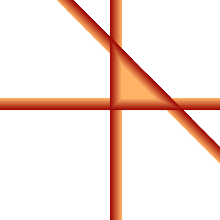
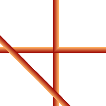
To explain what happens next, I have to introduce a new notion, that of the tangent cone at a vertex. The figures below should suffice to explain this. On the left is a 2D region defined by inequalities that are indicated by lines. On the right is an illustration of one of the vertices, along with its tangent cone.

Finding dimension is a purely local affair, so we don't have to worry any more with other vertices---we can throw away all those functions which are not $0$ at the given vertex. The region defined by the inequalities is now the tangent cone at the vertex. Apply the simplex method to maximize the last coordinate variable. If it is $0$, that variable is a constant $0$ on the cone, and may be discarded. Then try again with the new last variable.
Otherwise, it will be infinite, and there is a real edge of the cone leading away from our vertex along which this variable increases. In this case, discard all the functions which depend on this variable, and with the ones remaining, set it equal to $0$. We are in effect looking at a degenerate cone containing this edge, and we may replace this degenerate cone by a slice transverse to the edge, which is also a cone. The dimension of the original region is one more than the dimension of this new cone, and it is easy to see that we have for this cone also a coordinate system satisfying I and II.
In effect, we are looking at a series of recursive steps in which dimensions decrease at each step. Sooner or later we arrive at a region of dimension $1$, which is straightforward.
Final remarks
In a sequel, I'll look at the problem of listing all vertices of a polytope, in effect converting the specification of a polytope in terms of inequalities to its dual specification as the convex hull of its vertices.
Reading further
-
Hermann Minkowski, `Theorie der konvexen Körper, insbesondere Begründung ihres Oberflächenbegriffs', published only as item XXV in volume II of his Gesammelte Abhandlungen, Leipzig, 1911.
As far as I know, it was Minkowski who first examined convex sets in detail, maybe the first great mathematician to take them seriously.
-
Hermann Weyl, `The elementary theory of convex polytopes', pp. 3--18 in volume I of Contributions to the theory of to the theory of games, Annals of Mathematics Studies 21, Princeton University Press, 1950.
This is a translation by H. Kuhn of the original article `Elementare Theorie der konvexen Polyeder', Commentarii Mathematici Helvetici 17. 1935, pp. 290--306. At this time, game theory and linear programing had just made the subject of convex polytopes both interesting and practical.
-
Vašek Chvátal. Linear programming, W. H. Freeman, 1983.
This is the classic textbook. Somewhat verbose for someone who is already familiar with linear algebra, but still worth reading.
-
Günter Ziegler, Lectures on polytopes, Springer, 1995.
A deservedly popular textbook, neither too elementary nor too difficult.
Notes
-
Points and vectors. Points are positions, expressed as $(x, y, z)$. Vectors are relative displacements, expressed as $[x,y,z]$. As they say in physics classes, vectors have no position. Vectors give rise to translations: $v$ shifts $P$ to $P + v$. So you can add vectors to each other, and you can add points and vectors. But you cannot legitimately add two points. The two notions are often confused, since the coordinates of a position are those of its displacement from the origin. But origins depend on a particular choice of coordinate system, so this is not an intrinsic identification.
-
Programs. Look at the web page LP-python.html.
Bill Casselman
University of British Columbia, Vancouver, Canada
Email Bill Casselman
