It Just Keeps Piling Up!
We'll start off by looking at three basic types of deposition. Much (but not everything) is known about them, and together they cover a wide range of real world phenomena...
 Bill Casselman
University of British Columbia, Vancouver, Canada
Email Bill Casselman
Introduction
Stuff keeps falling all the time. Rain falls everywhere, snow falls on the ground, snow falls on snow, river sediments fall on the ocean floor, and in industrial work all kinds of materials are laid down in a somewhat random manner on all kinds of other materials. The technical phrase is that stuff is deposited on other stuff, and the process involved is deposition. It is important to understand different deposition processes in nature and in industry. Of course real-world deposition can be very complicated, so mathematicians look at simplified (often extremely simplified) models. For example, in real life most depositions take place onto a surface, whereas in most mathematical models they take place onto a line, and already for these very simplified models what happens is often not easy to understand.
The effect of rainfall is very simple. Water is a liquid of low viscosity, which means that it flows freely. In practice, the effect is just to form a level surface of puddles. But other kinds of deposition exhibit some kind of stickiness, and it is this that makes things difficult.
We'll start off by looking at three basic types of deposition. Much (but not everything) is known about them, and together they cover a wide range of real world phenomena.
What are the basic types?
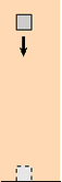
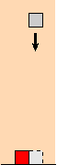
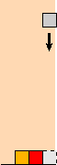
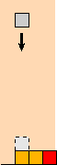
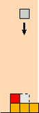
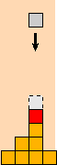
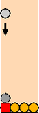
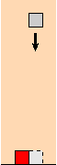
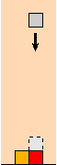
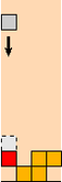
The three basic types of deposition we'll look at will have some features in common. First of all, the deposition will be onto a one-dimensional region of width $W$. At various times, a small square will appear somewhere in the sky above the region and fall onto whatever edge has already formed. What happens at that point depends on which type of process we are looking at. In each case, we ask, how do the stacks of squares grow?
We are looking at a finite region. Without some special assumption, something special can be expected at the boundary. To eliminate these effects, I'll assume the boundary to be circular, or in other words the process is periodic. We'll see what the consequences are in just a moment.
The time scale is normalized so that $W$ squares are dropped in $1$ unit of time. In $t$ units of time, the number of squares dropped is $Wt$.
Random deposition
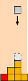
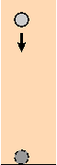
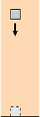
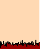
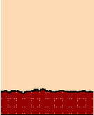
The simplest of all deposition processes is that in which the unit square just drops into place at the lowest unoccupied point. This is called random deposition. (The term 'random' is not all that justified. All the models we'll look at are random. For reasons that will become apparent, a better term might be `independently random'.)
This is not a type of deposition that occurs in nature, and it is too simple even to suggest what happens in nature, but it serves well as something to compare other processes to.
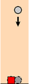
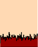
Random deposition with relaxation
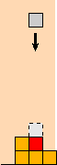
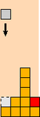
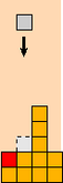
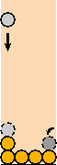
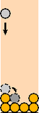
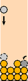
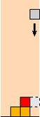
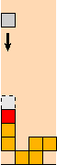
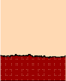
An interesting variation of this is one in which the square drops onto an unoccupied site, then drops into the nearest site that has minimum height. (If both sides are lower, it tosses a coin to choose.) The system tries to find minimal energy through purely local shifts. This is called random deposition with relaxation. In these figures, you can see how periodicity comes in.
It will fit intuition better if the squares are replaced by disks.
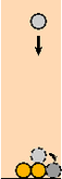
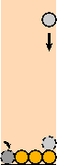
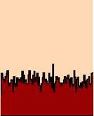
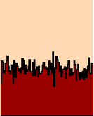
Ballistic deposition
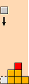
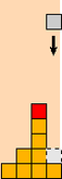
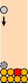
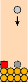
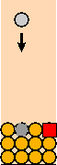
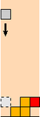
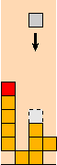
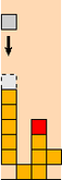
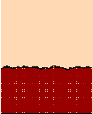
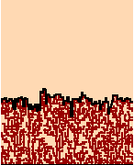
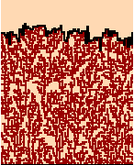
The most complicated of the three models is called ballistic deposition. In this, the square falls onto the first site where it sticks onto the first available neighbour. (The term `ballistic' is common in the literature. I have no idea why.) Here, to, periodicity should be apparent.
The problem
The problem is to figure out what the growing interface at the top looks like. In the real world, this is important because what actually interacts with the outside world is that growing interface, and one wants to deduce the underlying mechanisms from what one can see. One might hope to match a model one is familiar with.
We'll look now at some sample runs of each type.
Random deposition
Random deposition with relaxation
Ballistic deposition
Comments?
A closer look
Let's make another pass.
Random deposition
In this example, I start with a site of size $50$, dropping $40,000$ squares. On the left I have marked alternate generations with two colors.
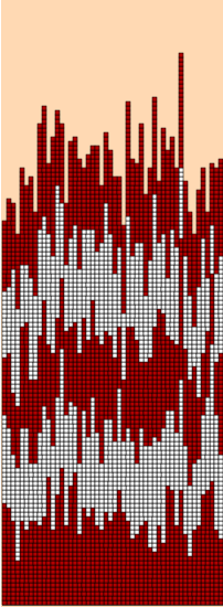
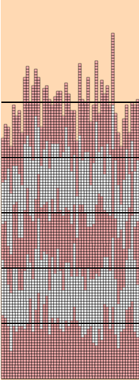
The heights of successive generations are very, very rough, but in some sense they grow uniformly. That is to say, the average height grows very uniformly. I show this in the right-hand figure, where horizontal lines indicate the averages of selected height distributions. The growth of the averages is very uniform, indeed. However, what is also happening as the stacks grow is that the size of the fluctuations from the mean also grows. This has a well-defined measure--the standard deviation: $$ \sigma^{2} = { \sum_{1}^{n} (x_{i} - \mu)^{2} \over n } \quad \hbox{ where $\mu$ is the mean } \quad { \sum_{1}^{n} x_{i} \over n }, \quad $$ Here is a table of time, mean, standard deviation: $$ \matrix { \hbox{t} & \mu & \sigma \cr 0 & 0 & 0 \cr 20 & 20.0 & 4.70 \cr 40 & 40.0 & 6.78 \cr 60 & 60.0 & 6.75 \cr 80 & 80.0 & 7.29 \cr 100 & 100.0 & 8.17 \cr } $$
Since $W$ squares fall in one unit of time, the average growth of the stacks can plausibly be expected to be at least roughly the same as the time elapsed. The table supports this hypothesis. But as far as the sizes of fluctuations in stack heights goes, all we can easily tell from the table is that they increase with time. We'd like to have a quantitative estimate of the rate of increase. But to do this with the run we are presently looking at would not be so informative, because the size of the base (i.e. $50$ sites) is not very large, and it turns out that quirky effects of small samples occur.
So I now make a run on a larger base, of size $500$, up to $t = 200$. We now plot a sequence of pairs $(t, \sigma)$ with $\Delta t = 10$ to see if we can guess how $\sigma$ depends on $t$:
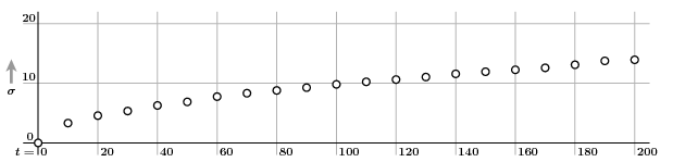
It looks like $s$ might be proportional to $\sqrt{t}$, say $s = c \sqrt{t}$. If so, then $\log s = \log c + (1/2) \log m$. We check this by plotting $\log \sigma$ against $\log t$:
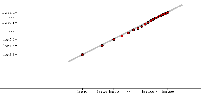
Sure enough, we see a line of slope $1/2$.
We can summarize: In the random deposition process, the average height of stacks grows with an approximately fixed velocity, but fluctuations in the height of stacks is large, and the standard deviation of the fluctuations is very near $\sqrt{t}$.
In fact, these claims can be rigourously proved. Each stack grows independently of every other stack, and grows something like the total number of 'heads' in tossing pennies. As the size of the base and the length of time for which the deposition proceeds, the fluctuations from the average $\mu = t$ are distributed very nearly according to the normal distribution $$ { 1 \over \sigma \sqrt{2 \pi} } \cdot \mathstrut e^{ -(x - \mu)^{2} \over \phantom{\big |} 2 \sigma^{2} } \quad \hbox{ with } \quad \sigma^{2} = t \, ( 1 - 1/W ) \, . $$
There is another way to see what is going on. In the common random walk, a particle starts off at the origin of a line, and at each subsequent time $i$ goes either one step backwards or one step forwards, each equally likely. In the process at hand, each stack can either remain the same, with probability $(W-1)/W$, or advance by one unit, with probability $1/W$. In other words, it is a kind of skewed random walk. This accounts for all we see. The important point is that the stack above each site behaves completely independently of every other stack.
Random deposition with relaxation
For the other deposition processes, the first question is, how do they differ from the random deposition?
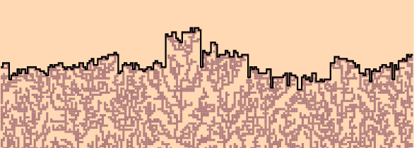
Here again is the relaxed deposition:
There are a number of things to observe. The first is that the process fills up the region below its top. It seems to progress with a uniform velocity, and in fact this velocity is essentially the same for all runs. The envelope of the growth is much, much smoother than it is for random deposition. Here is a typical scan:

A little thought will tell you that there are certain necessary features that explain the smoothness. Most important is that you will never see a jump of more than one in the scan. Furthermore, long successions of increments or decrements are rare, and you might therefore expect a lot of fairly flat segments, which is in fact what you see.
As with random deposition, an analysis of the standard deviation of interfaces is instructive.
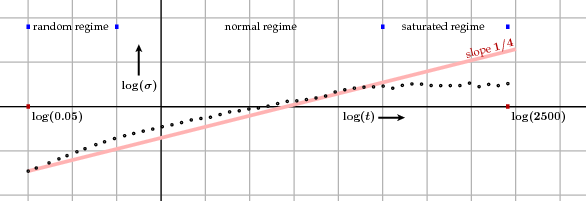
What we see here is a plot of standard deviation versus time, on a log-log graph. In this run, the number of sites was $100$, and the total elapsed time was $2500$, making $250,000$ drops in all. It happens, however, that individual runs exhibit a great deal of randomness that one might think to be inessential, so the data represents an average over many runs. The process divides roughly into three regimes: (1) The stacks are nearly all empty, and relaxation hardly plays a role; the process looks much like a random deposition. (2) What I call the normal regime, in which the standard deviation increases approximately proportionally to $t^{1/4}$. This is far more slowly than for random deposition. (3) A period in which the sites are in some sense in a steady state. During this saturated regime, which presumably goes on forever, the probability distribution of standard deviation remains more or less constant.
What does 'saturated' mean? Unlike with random deposition, neighbouring sites are not independent of each other; the heights of stacks are correlated. Intuitively, the distance at which one site 'feels' another grows, until the correlation extends to roughly all sites. From that point on we are presumably looking at an essentially stationary process.
In a real physical process the number of sites can be enormous and the process approximates closely a limiting process, just as a random walk over a long time period approximates a continuous Brownian motion. The limit possesses a certain scale invariance and, based on a reasonable guess as to what it is, there are good theoretical reasons for seeing why the exponent $1/4$ appears. The limiting process is called the Edwards-Wilkinson process, after the physicists who discovered it. It also predicts when the cross-over between the various regimes takes place.
The continuous limit process is well understood, although how exactly discrete approximations relate to it are not. Many variations of this process can be imagined. It is asserted often that they all share the same continuous process but there seems to be little idea of how to prove this rigourously.
One mathematical question that immediately springs to mind is, how smooth are these interfaces?
Ballistic deposition
I now turn to the third process. The scale of its fluctuations lies somewhere between that of the two other processes.
I shan't give details as I did for the others, but computer experiments and some theoretical reasoning lead to the conjecture that standard deviation is proportional to $t^{1/3}$. But whereas the distribution of the other fluctuations is known or at least conjectured to be normal, the distribution here is likely to be that first defined by the mathematicians Craig Tracy and Harold Widom in a totally different context. This is an extremely active topic of research, part of ongoing exploration of what is called Kardar-Parisi-Zhang (KPZ) universality, which is all about figuring out what processes give rise to similar distributions. Verifying particular cases, even experimentally, is not easy.
Comments?
More ... ?
One might consider a mathematical version of TETRIS®. There are seven basic shapes, called
tetrominoes.
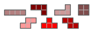
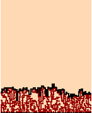
Every now and then, a random tetromino drops from the sky above a random site, after a random rotation. It falls as far as it can. (In this theoretical game, no rows are deleted.)
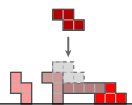
And here is what the result looks like, after a while:
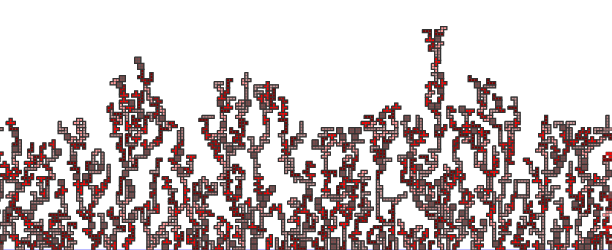
There is much in common with the other deposition schemes we have seen, particularly ballistic. In particular, a small amount of experiment indicates that the interface travels overall with a velocity essentially independent of any particular run involved. But, as Ivan Corwin asks, how much in other ways? For example, it seems that the fluctuations here are measurably wilder than those for ballistic deposition. As far as I know, there has not been any serious exploration of the question. The point is to try to see how universal KPZ universality actually is.
Anybody contemplating this question should first read the note by Farmudi and Vvedensky referred to below.
Comments?
Reading further
The popular literature on this subject is sparse and often misleading. This is forgiveable, because the mathematics involved is very difficult.
-
A-L. Barabási and H. E. Stanley, Fractal concepts in surface growth, Cambridge University Press, 1995.
This is the standard text in the subject, and it is quite readable, although not mathematically deep. But it looks to me as though many of the diagrams of simulations are not accurate, or perhaps not labeled accurately. For one example, I have never seen data as 'good' as those in Figure 2.3 on a single run, so this probably illustrates an average of several runs. For another, all of the interfaces of the graph of the simulation of random deposition with relaxation in Figure 5.2 look far too rough. Among other things, they seem to have several jumps of more than two steps, which is impossible for the simulation they describe. So the simulation in play is perhaps one with relaxation to just a nearest neighbour.
Random deposition is treated in Chapter 4, random deposition with relaxation is discussed in Chapter 5, and ballistic deposition in Chapters 6-7.
-
Ivan Corwin, Kardar-Parisi-Zhang universality, NOTICES of the American Mathematical Society, March 2016.
Corwin has written many surveys of this subject. This is the most recent. This article was my initial stimulus to try to learn about the subject of depositions, and Corwin has offered me much useful help. He is of course not to be blamed for my misconceptions.
-
Bahman Farmudi and Dimitri Vvedensky, Large-scale simulations of ballistic deposition: the approach to asymptotic scaling, Physical Review E 83 020103 (2011)
This is the most thorough discussion I have seen of the enormous amount of computation necessary to get really good estimates of parameters of deposition processes. It is not cheerful reading, but the problem it presents, of understanding exactly why computations are so taxing, is intriguing.
Bill Casselman
University of British Columbia, Vancouver, Canada
Email Bill Casselman