Introduction
We would all love to be able to see into the future. It would be great to know what the weather will be, if we are putting enough money aside for retirement, how our friendships will turn out, or if a decision about what to study in college will bring happiness. It turns out that using mathematics may be more effective than using a crystal ball for helping see into the future. We all enjoy when nice times come our way and try to avoid unpleasant times. However, in everything humans do there are risks for negative consequences and we all seek ways to soften those risks. Often mathematics can help.
Crystal ball, courtesy of Wikipedia
This column honors the theme of Mathematics Awareness Month for 2016, The Future of Prediction. More about previous themes is available on the Mathematics Awareness Month website.
There are very few places in the world where there are no "external" risks to humans who want to lead trouble-free lives. Thus, in the United States some parts are prone to tornadoes, large snow falls, others to coastal flooding, hurricanes, river flooding and earthquakes. In areas where loss of life and property might occur due to these "acts of nature," it would be nice if predictions would make it possible for loss of life to be avoided altogether and property damage be kept to a minimum. Mathematical models have been developed that assist with all aspects of natural disasters. The most common we rely on are the increasingly accurate week-long weather reports that are provided, among others, by the National Weather Service. These forecasts are created using data from satellites and land-based monitoring and sensor systems. They also rely on models of the atmosphere that are rooted in the theory of partial differential equations and numerical methods for solving these equations. Computing power and progress in theory have gone a long way to making these reports much more reliable.
A interesting example of the concerns about avoiding danger from acts of nature was the trial of a group of Italian geologists and a government official for allegedly failing to give proper warning about an earthquake that killed 309 people in L'Aquila, Italy in 2009. Geologists around the world expressed concern that while progress had been made about trying to forecast earthquakes, there were no certainties only probabilities in the forecasts that could be made. After a trial, seven individuals were found guilty of manslaughter and sentenced to six years in jail. In 2014 an appeals court freed the geologists and reduced the sentence of the government official to the relief of scientists around the world but citizens in the courtroom who were relatives of the those who died in L'Aquila decried that the "government" had exonerated itself.
When a major storm approaches, can weather forecasters be blamed if they don't warn of the potential dangers strongly enough? Sometimes due to forecasts, transportation systems that might be damaged by a major storm are shut down preemptively, causing great logistical and economic hardship to many people. If the storm doesn't materialize, as sometimes has occurred, this is frustrating to many, but the flip side, not responding strongly enough when lives might be saved, is the issue involved in what happened in Italy with regard to the earthquake forecast. Compared with weather forecasting, the forecasting of earthquakes is much less advanced.
Similar issues come up every year (or sometimes in multiple year cycles) when certain infectious diseases (e.g. flu) make the rounds. For the young, getting an illness like whooping cough or measles can cause death. For the elderly, it is unclear if some of the vaccinations they had in their youth still are efficacious and then there is the flu, which affects the elderly in a serious way. Whereas getting the flu for younger people is disruptive, for the elderly catching the flu can lead to pneumonia or be life threatening in other ways. So should parents vaccinate their kids and should the elderly get flu shots? Some people get allergic reactions to vaccines but the long term history of vaccinations is to have significantly improved the life expectancy and quality of life for many.
Risky behavior
Recently there was a staggering large lottery prize of 1.6 billion dollars for the US Powerball Lottery. One reason to have faith in the mathematics of lotteries and casino gambling is that these "businesses" thrive just as long as they have lots of customers! If one had a crystal ball that helped pick the right lottery ticket, one could get a lot of income.
When thinking about the future either as an individual or part of a group one often has expectations for the future--sometimes good expectations and sometimes ones that seem much less appealing. One contribution of mathematics to understanding what the future might bring is the notion of expected value. When mathematicians use this term they have a very precise idea in mind but it is an idea which has many subtleties. One reason people are nervous about the future is that they are unsure what will happen in the future. The future seems to involve chance, randomness, stochasticness, and probability. In order to understand what is meant by expected value, we first have to say something about probability theory.
We commonly hear expressions about the future similar to the following:
The probability of rain is 70 percent.
The chance of having another earthquake in this location is 1 in a million.
When a pair of "fair" dice are rolled the chance that the sum of the spots on the two dice will be a 7 is 1/6.
What do statements of this kind mean? To answer this question one has to come back to the two pillars of mathematics--theoretical mathematics and applied mathematics. Theoretical mathematics builds up systems of ideas and concepts based on definitions and axioms (rule systems) and then deduces mathematical facts, theorems, from these constructs. Applied mathematics takes these mathematical systems and tries to use them to get insights into the world. I will try to proceed in a relatively informal manner, trying to avoid "heavy" mathematical notation and "formal" definitions.
First of all, probability is used both in domains with finitely many outcomes and in those with infinitely many outcomes. To help build intuition I will look at the theory by using contexts to try to get the idea across. If Susan is expecting twins, there are four possibilities for the birth order of children: a boy followed by a boy, a girl followed by a girl, a boy followed by a girl, and a girl followed by a boy. One might ask about simultaneous births as being other "alternatives" but we will consider only the four possibilities mentioned. In a different context we might catch a salmon going to its spawning ground in a certain river in the Western United States, and weigh this salmon. The possible outcome now is a real number in a certain range of weights that salmon can display--the weight can be one of an infinite number of outcomes. From a mathematical point of view we can try to model these possibilities by imagining a set M of outcomes from some kind of "experiment" or observation of the world. The set M can be finite or it can be infinite. To each outcome m in a finite set of outcomes I will assign a real number called the probability of outcome m and I will denote that probability by P(m). These numbers can't be assigned in a totally arbitrary way--they most obey certain properties or axioms:
a. P(m) takes on values between 0 and 1 including 0 and 1.
b. The sum of the values P(m) for all of the m in M add to 1.
Note that if the probability of m occurring is P(m) then the probability of the complementary event, m', that m will NOT occur is 1--P(m). If a coin can either come up heads or tails and the probability of a tail is 2/5, then the probability of a head is 3/5.
Note that because we only have a finite number of outcomes we don't need any idea related to limits (Calculus) to do the calculations.
For sets M with an infinite number of outcomes we will insist that the same two conditions as above hold. If there were a smallest value among the numbers P(m), then we could not have a sum of 1 for all the outcomes. Adding some finite number no matter how small infinitely often would result in a number bigger than 1. Thus, for infinite sets dealing with probabilities has additional subtleties. However, it is worth noting that one can find infinite sets where the probabilities of the outcomes for each individual event in the set can be nonzero. This can be true because there are infinite sequences of positive numbers whose sum is 1.
When mathematics is used in the world we have to interpret the meaning of the mathematical constructs outside of the world of undefined terms and axioms.
If one is given a collection of numbers, say the weights you have had for the last 30 days (perhaps taken at the same time every morning) one will see fluctuation in the numbers--they probably will not be the same. If one wants to get a sense of "pattern" for these numbers one approach is to compute some typical or "average" value. One very appealing such number is the mean. The mean, often called the average, is obtained by adding the numbers together and dividing by the number of measurements.
The trouble with using one single number to represent a large collection of numbers is that many different kinds of data sets may have that same single number as their representative. Thus, the mean of 5, 5, 5, 5, 5, 5 is 5 while the mean of -3, -3, -3, 13, 13, 13 is also 5. One of the early developments in using numbers in science and statistics was to realize that taking the same measurement "independently" several times might be a way to get a more reliable value for the number than just measuring a quantity once. Whenever a measurement is taken there will inevitably be some errors due to the measuring device and "human" procedure but one can try to make measurements as reliable as possible.
The analogue of the mean for values that are subject to chance is a quantity called the expected value. Suppose in a game that there is a 3/10 chance of winning $3 and a 7/10 chance of winning $4. One can see on "average" what will happen if you play such a game, by weighting the outcomes with the probabilities of the outcomes.
Thus for the situation above the expected value is that you will get $3, 3/10 of the time and $4, 7/10 of the time so:
Expected value = 3(3/10) + 4(7/10) = (9/10) + (28/10) = 37/10 = 3.70
If to play this "game" you needed to pay $3.75 on average you would expect to lose 5 cents on average every time you played. Sometimes you would lose 75 cents, when you won $3 and sometimes you would gain 25 cents by winning $4 but because you don't win and lose equally often, the probabilities of the outcomes are not the same, you will on average lose 5 cents. Note that 3.70 is not an outcome from playing the game and that 3.70 is not a probability.
Sometimes the way "experiments" unfold affects the probability of an event.
Consider these two different regimensIf involving an urn with two black balls and two white balls:
Case A. Select a ball from the urn after stirring the contents of the urn; then select a second ball after replacing the first ball (whose color is noted) and stirring the urn again.
Case B. Select two balls from the urn after stirring, one ball after the other.
Not surprisingly, the probability of the event that you get two balls which are black depends of which of these two procedures you use. In Case B if the first ball you draw is white, it is not possible to get a pair of black balls.
For Case A, you get two black balls only if the first drawing is a black ball and the second ball is also black. So the probability of BB (B for black on the first selection B on the second selection) can be computed by P(BB) is (1/2)(1/2) = 1/4. In case B to do the computation we need to analyze the situation this way:
The first ball drawn was black and the second ball was black as well.
So the chance that the first ball is black is 2/4 = 1/2. Now since there are only three balls left, one black and two white, there is a 1/3 chance the second ball drawn is black.
Taking this into account we see that the probability of two black balls being drawn is (1/2)(1/3) = 1/6.
This simple environment involves one of the most fundamental but subtle issues of probability theory, that of conditional probabilities. This notion dates to the earliest days of the study of chance. Using modern notation we write P(A|B) to denote the probability that A occurs given that B occurred. For example, the probability that when two balls are drawn from an urn the second ball is black given that the first ball is white in the situation we just described, would be 2/3. We also can think of P(A|B) as being the same as P(A and B)/P(B) = P(first ball is black and the second ball is black)/(P(second ball is black) = (1/3)/(1/2) = 2/3.
How can one "define" or think of the value of P(X|Y)? In words, we seek the probability that if Y happens then X happened, so P(X|Y) is the probability that X and Y happened divided by the probability that Y happened. Note that P(Y) is in the denominator for this calculation. For P(Y|X) we compute the probability that Y and X happened (which is the same as the probability that X and Y happened) but we divide by P(X). We are finding "what part of X" is contributed to by "Y and X."
Many people get confused between the two conditional probabilities P(A|B) and P(B|A) which are typically not the same. Thus, if A is the event that a certain medical test is positive and B is the event that the patient has the disease it is very different to know the probability that if one has the disease the test result will be positive versus the probability that if the test result is positive one has the disease!
A medical test can be very accurate, but when a disease is relatively rare, just because one tests positive this does not mean that it is almost certain that one has the disease. A numerical example will help show the issues involved.
Suppose that a disease (D) is quite rare in the sense that the chance that a person in the general population will have it is .005, 5 people in 1000. Suppose that a diagnostic test for disease D, perhaps a blood test, returns an indication that the patient has disease D with probability .99, when the disease is present. Unfortunately, there is also a chance the test will give a positive result when the disease is NOT present, and this probability is .05, relatively low. Note that .99 and .05 don't add to one because these two events are not complementary. We are given three different numbers here, and we will use these numbers to generate a variety of other numbers which are deduced via the "rules" by which probabilities are used. Let me introduce some notation to try to sort out what is happening. In a situation of this kind the notation is both a blessing and a curse. It allows one to be precise because there are similar sounding but different ideas swirling around but a lot of symbols are necessary to capture the distinctions involved.
Let
-
T denote the event of getting a positive test result, whether or not the disease is present,
-
P(D) denote the probability that a particular person will have the disease,
-
P(T|D) the probability a person will test positive when the disease is present, and
-
P(T|D') the probability that a person will test positive in spite of the fact that the disease is NOT present.
With the information above we can write down the values of these three different probabilities:
P(D) = .005
P(T|D) = .99
P(T|D') = .05
The patient is interested in knowing the chance that he/she has the disease when the results of the test are positive, P(D|T), but note that this is NOT one of the numbers that is given above! However, the results of probability allow one to deduce this number.
In addition to other tools of probability we will make use of a "fact" known as Bayes's Theorem or Bayes's Formula, a result developed by Thomas Bayes (1702-1761) but not published in his lifetime. In modern times Bayes is honored in statistics by the use of the terms Bayesian inference and Bayesian statistics.
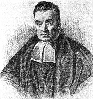
Portrait of the Reverend Thomas Bayes's
The result due to Bayes is spelled out in "neon" lights below.
Bayes's Theorem. (Image courtesy of Wikipedia.)
Though we may only know P(B|A) (and other information) this result allows us to compute the other conditional probability associated with the problem P(B|A).
Returning to our diagnosis situation above, let us see what we can deduce.
First, using the notation of the complement of events, and that complementary events' probabilities sum to 1, we have
P(D') = 1-P(D) = 1-.0005 = .995 (the chance that a particular person will not have the disease)
P(T'|D) = 1-P(T|D) = 1-.99 = .01 (the chance that a particular person who has the disease will not test positive)
P(T'|D') = 1-P(T|D') = 1-.05 = .95 (the chance that if the disease is not present, a particular person will not test positive).
Now, let us get some of the other probabilities that are of interest, to begin with the probability of getting a positive test result whether or not one has the disease, and the probability of getting a negative result whether or not one has the disease.
The probability of getting a positive test result can come about in two ways: one can have the disease and get a positive test result and one can not have the disease and get a positive test result. In symbols we can write:
P(T) = P(T|D)P(D) + P(T|D')P(D') = (.99)(.005) + (.05)(.995) = .00495 + .04975 = .0547
Now,
P(T') = P(T'|D)P(D) + P(T'|D')P(D') = (.01)(.005) + (.95)(.995) = .9453
(where we are adding together the probabilities that a person had the disease but did not test positive to the probability that the person did not have the disease and did not test positive.
Note as a check that we did the calculations properly, .0547 + .9453 should add to one and they do! Perhaps these numbers seem surprising--getting a positive test result is rare but this reflects the fact that few people have the ailment.
But so far, we have not gotten the number we really are interested in. What is the chance that the person has the disease if that person tests positive? How scared should a person with a positive result be? This is where we need to use Bayes's result.
P(D|T) = (P(T|D))(P(D))/P(T) = (.99)(.005)/(.0547) = .0904936 = .0905
Thus, only a small part of those who test positive actually have the disease even though the test detects the disease with high probability. This is true because the disease iis so rare. Typically, one would now do another independent test to see if the disease is really present or not, so as to avoid unnecessary treatment.
Bayes's result can be used to get three other conditional probabilities, two of which can also be gotten by using the fact that events that are complementary have probabilities that add to 1.
These other numbers are:
P(D'|T) = .9095
P(D'|T') = .99995
P(D|T') = .00005
This last number can be computed using Bayes's result as follows:
P(D|T') = (P(T'|D))(P(D))/P(T') = .01(.005)/ .9453 = .00005
Yes, a sea of calculations and symbols, but ones that help a patient and his/her physician put in perspective what it means to get positive result on a test for a rare disease.
Comments?
Stars of probability theory and statistics
With hindsight one can see what happened in the world after the present moves to the future, and what had been the present becomes the past. What follows is a vastly oversimplified look at how probability evolved as a mathematical subject but it shows that mathematical investigations involving probability were not confined to one country nor always to mathematicians who are widely known for contributions to other parts of mathematics. Also from the earliest beginnings of attempts to get insight into chance and probabilistic ideas, there were two different strands to the ideas. One strand had to do with how to decide how likely or probable something was based on knowledge or evidence (will a certain hurricane hit New York City) and the behavior of systems which involve "chance" such as when coins are tossed or dice are thrown. In one perspective if one knew all of the information to invoke the laws of physics to spinners, coins tosses, and dice throws, the specific outcome each time could be known, but in practice this is not possible. Yet, there are "regularity" patterns associated with such processes which are in part the subject matter of probability theory. If a pair of fair dice are tossed, what portion of the time will one see the sum of the dots on the dice added to 4?
While almost surely those with mathematical talent thought about "chance" in older times, the contribution Gerolamo Cardano (1501-1576) made has come down to us. Cardano looked into issues which today would be considered parts of combinatorics, the part of mathematics concerned with counting problems. He studied the patterns of outcomes which would occur when three different dice were tossed and one might want to count the number of different ways that a 8 or 9 might occur. However Cardano was not the first or last to make "errors" from a modern perspective. Thus, when a (fair) coin is tossed twice we can code the outcomes of head (H) and tail (T) by the sequences HH, HT, TH, and TT, where HT and TH. by way of example, denote that the first toss was a head and the second a tail, and that the second was a tail and the first was a head, respectively. If we count the number of heads that can occur, the answer can be 0, 1, or 2 but today it would seem strange to argue that these three outcomes were equally likely, and that P(0 heads) = P(1 head) = P(2 heads) = 1/3. Rather we would say that the probability of exactly one head in two tosses would be 1/2 while the probability of two heads and two tails are each 1/4. However, this seemingly simple error was not uncommon in the early days of combinatorics and probability theory. Things are more transparent in hindsight. The "modern" origins of the study of chance with a mathematical basis dates to the work of Blaise Pascal (1623-1662) and Pierre de Fermat (1601-1665). In 1654 Pascal and Fermat had correspondence that dealt with chance issues related to a gambling game.
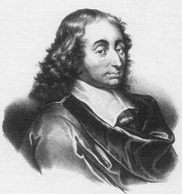
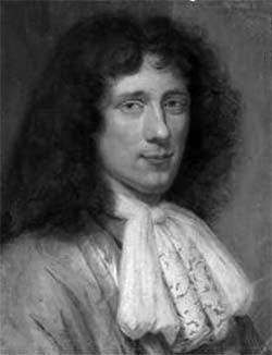
Portrait of Blaise Pascal
It is intriguing that Pascal both addresses a fair way to divide the stakes in a gambling situation that was interrupted and could not be brought to a conclusion (in his correspondence with Fermat) as well as a "bet" on the existence of God. Whereas modern decision theory might be used to determine whether or not to conduct drilling for oil in a particular underwater site, Pascal used a surprisingly "modern" analysis of why someone might want to believe in God. The discussion here follows the ideas that Pascal developed in his famous philosophical treatise, the Pensées. God either exists or does not exist. Every person must decide what his/her position on this question, and one can't just "not decide." Reason alone cannot answer the question of whether or not God exists. Presumably there is a finite probability that God does exist. One can examine the consequences to you from which position you decide to adhere to. Pascal suggests one should live as if God exists and seek God because if God exists the gain is "infinite" and if God does not exist one loses out on relatively little by one's belief. While some find Pascal's argument persuasive, others do not.
The first "book" about probability seems to have been written by Christiaan Huygens (1629-1695).
Portrait of Christiaan Huygens
As was true in those times the book was published in Latin. De ratiociniis in ludo aleae appeared in 1657 as an "appendix" to Frans van Schooten's Exercitationum Mathematicarum Libri Quinque and thus had a limited impact beyond the growing but small group of intellectuals who were developing the ideas and tools of modern science and mathematics.
Relatively soon after this work, ideas related to chance and statistics drew the attention of John Graunt (1620-1674) to data about illness which could be used to protect oneself against what the future might bring, in particular the consequences of epidemics. Graunt's work probably would today be said to be related to the scholarly field of demography. He constructed a table, whose modern descendant is the "life table" used by insurance companies to set the premiums for life insurance. Sixty-year-olds are more likely to die within a specified period of time than a 30-year-old, so in setting the price that someone should pay to buy a life insurance policy one uses life tables. With time it has been realized that not all people live the same amount of time beyond their age at a given time. Thus, women are more likely to live longer, given they have achieved a given age. Furthermore, smokers are "on average" less likely to live as long as people who don't smoke.
Many important developments occurred during the 18th century. Jacob Bernoulli in "Ars Conjectandi" discussed what today would be called the law of "large numbers." The idea that if one takes a sample of measurements which are generated "independently," then as the number of measurements grows the mean of these measurements gets more "stable." Thus, if one conducts a sequence of tosses of a "fair" die, where the number of spots is 1, 2, 3, 4, 5, or 6, then with more and more tosses, the mean value of the number of spots gets closer and closer to 7/2 (which is (1+2+3+4+5+6)/6). Bernoulli is honored today with the term Bernoulli trials, a special probability model (binomial distribution) where there are exactly two outcomes when an experiment is performed, as in the case of coin tossing (outcomes of heads or tails), or observing the sex of a large number of mice (outcomes of male or female). Abraham de Moivre during this period not only looked at the financial instruments known as annuities but the use of what today is called the "normal" distribution to approximate the binomial distribution.
Pierre de Simon Laplace (1749-1827) did work in probability that "summarized" and extended much of what had come before. Laplace not only made important contributions to probability but to nearly all parts of mathematics. An early contribution was his "memoir" in 1774 on what is sometimes called "inverse probability" where he was led to the same kind of ideas that Bayes had looked at. His contributions to probability were published in his Mémoire sur la probabilité des causes par les événements (1774). In some of his work Laplace emphasized what today would be called the "equiprobable" model, in which although the probabilities of certain events are unknown, they are assumed to be equally likely. Often this is not always reasonable because though one may not know the probabilities of what might happen, one can be sure that some are more likely than others.
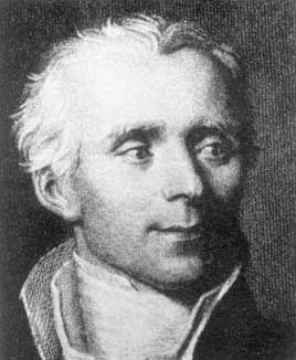
Portrait of Pierre Simon Laplace
Others in the 19th century contributed to ideas in probability and statistics. These included Gauss (1777-1855) and Adrien-Marie Legendre (1752-1833) (a pioneer in the use of least squares techniques for fitting a curve to a set of observations and to trying to extrapolate these observations into the future).
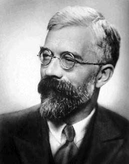
However, as time went on it became clear that as a mathematical subject, probability theory had to be put on a more "axiomatic" foundation. Without clear definitions and precise frameworks to prove results some concerns had emerged about the foundations of probability theory. One person who rose to this challenge was the Russian/Soviet mathematician Andrey Kolmogorov (1903-1987). Kolmogorov's contributions to mathematics were extremely wide ranging including his work on homology and cohomology.
Photograph of Andrey Kolmogorov
With the tremendous growth in the development of the sciences and mathematics late in the 19th century and beyond, attempts were made to use mathematical ideas related to probability and statistics not only in the sciences but in other fields. Though probability and statistics were increasingly being placed on a better theoretical foundation and proofs of fundamental results were being proved that stood up to modern standards of rigor (the law of large numbers, the central limit theorem, etc.), controversy broke out about the methodology that was used to get reliable insights into the world based on probability and statistical methods. As noted before some of this was related to the difference between when someone talked about the probability that drug A was better than drug B as compared with the probability that there would be another accident of the kind that had happened at Chernobyl (1986), Three-Mile Island (1979), or Fukushima (2011). Certain kinds of experiments can be repeated and the results tabulated but other events don't have that character.
In the last 125 years there have been a variety of mathematically trained scholars who developed "statistical" tools for drawing inferences from data. Below is a group of photos and very brief comments about a sample of such contributors to statistical testing.
Karl Pearson (1857-1936) helped lay down the modern theory of statistical testing. He investigated procedures for conducting statistical hypothesis testing theory (including the use of the chi-square test) and provided arguments for how to make decisions when faced with different alternatives in a systematic way.

Photograph of Karl Pearson
Jerzy Neyman (1894-1981) was born in Poland but spent a large part of his career in the United States. While in the US he taught at the University of California, Berkeley, where he supervised 39 doctoral students. His name is often tied to that of Karl Pearson for his work on hypothesis testing methodology and he helped encourage the use of confidence intervals (1937) as part of the process of carrying out statistical studies.
Photograph of Jerzy Neyman
Another pioneer of trying to use statistical methods to get insight into genetics (evolution) and other subjects was Udny Yule (1871-1951). Yule wrote some influential papers on time series, where one tries to understand data from measurements taken at the equally-spaced time intervals. Yule and Pearson were often at odds with exactly what approaches and interpretations to give to statistical issues. Yule taught statistics at Cambridge University for 20 years.

Photograph of Udny Yule
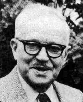
Another important pioneer of statistical methodology was Ronald Aylmer Fisher (1890-1962), who encouraged the use of mathematical models for studying genetics and evolution. In 1935 he wrote a book called The Design of Experiments where he discussed the use of what today are called block designs and balanced incomplete block designs for use in agricultural work and other environments where one wanted to minimize chance variation affecting the results of a study. Thus, variations in fertility in different parts of a field could be "corrected for" by planting the different varieties of plants in an experimental study of their yields using block designs. Fisher talked about the use of a p-value in conjunction with various statistical testing procedures but almost certainly would have been appalled by the mindless approach to claiming that "significant" results were obtained because as part of a poorly designed study a calculation obtained resulted in a small p-value.
Photograph of Ronald Fisher
As one group of scholars was evolving statistical testing procedures for extracting information from data, another group of mathematically inclined individuals was trying to sort out the foundations for being able to use probability theory in the world in the many different settings where it would be of value to assign probabilities to events. Again these individuals had many national origins and very varied careers. Loosely speaking these individuals are associated with thinking of probabilities in what some call a "subjective" framework rather than in a "frequentist" view. Again, there are situations where it makes some sense to intuitively regard probabilities as "stabilized" values of relative frequencies as the number of repeats for some "experiment" increases. In other situations this way of approaching probabilities is not supportable. So there is also a school of probabilists who think of probabilities of as "degrees of belief" but not all people who adopt this point of view agree exactly on what probabilities and/or degrees of belief mean!
Frank Ramsey (1903-1930) is probably best known for Ramsey's Theorem in combinatorics but he also wrote a series of important papers on probability theory and utility theory (1926). In this work he offered views of probability and making decisions under uncertainty that are now generally described as "bayesian methods." Given the unusual creativity that Ramsey brought to what he did it is especially tragic that he died at such a young age.
Photograph of Frank Ramsey
Bruno de Finetti (1906-1985) also developed ideas about probability that were "subjective" and based on degree/intensity of belief. De Finetti was born in Austria but spent much of his career in Italy.
Photograph of Bruno de Finetti
Probably the most influential of those who emphasized a subjective approach to probability was Leonard Jimmie Savage (1917-1971) though his last name at birth was Leonard Ogashevitz. Savage wrote extensively about the foundations of statistics and also applied his ideas about using subjective probabilities in game theory and decision making. Savage developed the idea of using a mini/maxi view involving regret in making decisions. The idea is to make computations for each of the different actions a player in a game against nature might make not by using the player's utilities. Rather make the computation in terms of regret, the discrepancy between what would occur if for a particular state of nature one chooses some other action than the best action available. If an action A for state of nature N yields -3 but for the same state N one could have gotten 5 from a different action, the the regret for action A is 8. For any state of nature, the regret for the best action would be 0. In conjunction with his statistical and game theory work Savage worked with a variety of economists, including Milton Friedman.

Photograph of Leonard Jimmie Savage
Very recently, there has been renewed concern about the methodology of using a "formulaic" approach to using hypothesis testing in psychology, medical studies, and other realms where statistical methods are being used to increase our knowledge. Some have argued that p-values are being used in a mindless way that does not always give rise to results that other researchers can replicate. Two blogs which regularly treat the issues here are maintained by the statistician Andrew Gelman (Statistical modeling, Causal Inference and Social Science) and the philosopher Deborah Mayo (Error Statistics Philosophy).
The bottom line is that it would be nice to have a reliable crystal ball for understanding the world that is and the world that will be. Mathematicians, statisticians, and other scholars are working hard to bring us all better futures.
Comments?
References
Beniston, M,, From Turbulence to Climate: Numerical Investigations of the Atmosphere with a Hierarchy of Models, Springer, Berlin, 1998.
Daston, L., Classical Probability During the Enlightenment, Princeton U. Press, Princeton, 1988.
Falk, R., and M. Bar-Hillel, Probabilistic dependence between events. The Two-Year College Mathematics Journal. 14 (1983) 240-7.
Falk, R., Conditional probabilities: insights and difficulties. In Proceedings of the Second International Conference on Teaching Statistics 1986, pp 292-297.
Falk, R., Misconceptions of statistical significance. Journal of structural learning. March, 1986.
Gelman, A. and J. Carlin, H. Stern, D. Rubin, Bayesian Data Analysis (2nd edition), Chapman & Hall/CRC, Philadelphia, 2003
Hacking, I., The Emergence of Probability, Cambridge U. Press, New York, 2006.
Hald, A., A History of Mathematical Statistics from 1750 to 1930, Wiley, New York, 1998.
Hald, A., A History of Probability and Statistics and Their Applications Before 1750., Wiley, New York, 2003.
Mayo, D., Experimental Knowledge, University of Chicago Press, Chicago, 1996.
Mayo, D., Error and Inference: Recent Exchanges on Experimental Reasoning, Reliability, and the Objectivity and Rationality of Science, Cambridge University Press, New York, 2010.
Roulstone, I. and J. Norbury, Invisible in the Storm: the role of mathematics in understanding weather, Princeton U. Press, Princeton, 2013.
Stigler, S., The History of Statistics: The Measurement of Uncertainty Before 1900, Harvard U. Press, Cambridge, 1990.
van Plato, J., Creating Modern Probability: Its Mathematics, Physics and Philosophy in Historical Perspective, Cambridge U. Press, New York, 1994.
Those who can access JSTOR can find some of the papers mentioned above there. For those with access, the American Mathematical Society's MathSciNet can be used to get additional bibliographic information and reviews of some these materials. Some of the items above can be found via the ACM Portal, which also provides bibliographic services.
 Joseph Malkevitch
York College (CUNY)
Email Joseph Malkevitch