Untangling Your Square Dance
In this article, we will describe a one-to-one correspondence between rational tangles and the rational numbers and see how the process of untwisting a rational tangle is related to the Euclidean algorithm. ...
Introduction
It is sometimes said that mathematics is about recognizing and describing patterns. What is surprising is how similar patterns arise in seemingly disparate areas. In this column, we will look at rational tangles, which appear as useful building blocks in the topological theory of knots, and see how these tangles may be described using number-theoretic ideas. In particular, we will see how the Euclidean algorithm, one of the oldest known algorithms in use, provides a means of understanding rational tangles.
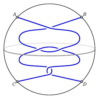
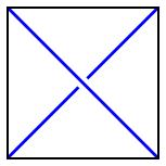
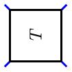
We obtain a tangle by tying a few pieces of string inside a three-dimensional ball so that any free ends are on the boundary of the ball. Since the tangle below has two strands that meet the boundary in the four points $A$, $B$, $C$, and $D$, we call it a 2-tangle.
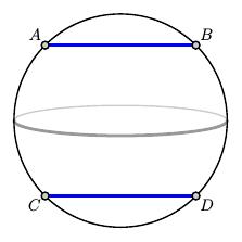
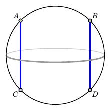
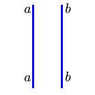
There are two elementary 2-tangles consisting simply of two horizontal or two vertical strands.
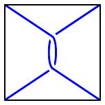
A rational tangle is a special kind of 2-tangle that may be unwound into one of the two elementary 2-tangles by twisting the endpoints. For instance, the tangle above is a rational tangle; if we twist $A$ and $C$ around one another, we obtain the tangle below. It should be clear how to continue unwinding from here.
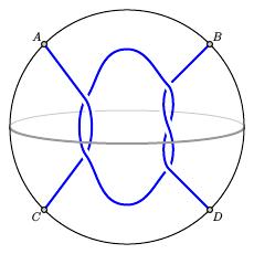
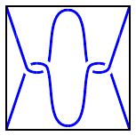
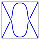
Not every 2-tangle is rational as the examples below show. For instance, the 2-tangle on the left has a third component in the middle; a little experimentation shows that the tangle on the right cannot be unwound by twisting.
We will usually represent tangles by a two-dimensional diagram drawn in a "tangle box."
Two tangles are considered equivalent if they are isotopic to one another; simply said, we may deform one tangle into the other by moving the strands without one crossing through the other, and without moving the endpoints. If tangles $T_1$ and $T_2$ are isotopic, like the two below, we write $T_1\sim T_2$.
Conway recognized that rational tangles serve as basic units in the construction of knots and used them to create a systematic notation for knots and to develop a list of all knots having 11 or fewer crossings.
In this article, we will describe a one-to-one correspondence between rational tangles and the rational numbers and see how the process of untwisting a rational tangle is related to the Euclidean algorithm.
Operations on rational tangles
We may form new tangles from old ones using a few natural operations. In this way, we will find a simple way to create and represent all rational tangles.
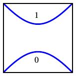
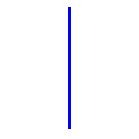
To begin, we will denote the following tangles by $[0]$ and $[\infty]$.
 |
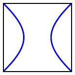 |
| $[0]$ |
$[\infty]$ |
Beginning with $[0]$, we may twist the rightmost endpoints to obtain tangles $[1]$ and $[-1]$ depending on the direction of the twist.
 |
 |
| $[1]$ |
$[-1]$ |
Given tangles $T$ and $S$,
we will define operations
- addition: the tangle $T+S$ is
- multiplication: the tangle $T*S$ is
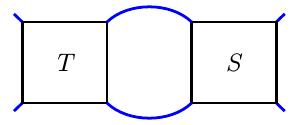
For instance, if $T$ and $S$ are
 |
 |
| $T$ |
$S$ |
then the sum and product are
 |
 |
| $T+S$ |
$T*S$ |
We may also see, for instance, that $[1] + [-1] = [0]$.
|
$+$ |
|
$=$ |
 |
| $[1]$ |
|
$[-1]$ |
|
$[0]$ |
Also, we may define $[1]+[1] = [2]$ and so forth.
|
$+$ |
|
$=$ |
 |
$=$ |
 |
| $[1]$ |
|
$[1]$ |
|
$[2]$ |
More generally, we define $[1] + [1] + \ldots + [1] = [n]$; for instance, the tangle $[5]$ is shown below.
 |
| $[5]$ |
For reasons that will become clear later, we will denote $[1] * [1] = 1/[2]$.
|
$*$ |
|
$=$ |
 |
$=$ |
 |
| $[1]$ |
|
$[1]$ |
|
$1/[2]$ |
We likewise have $[1]*[1]*\ldots*[1]=1/[n]$.
 |
| $1/[5]$ |
If $n=0$, we have $1/[0] = [\infty]$.
Using these operations, we may write rational tangles in a standard form. We begin with either $[0]$ and $[\infty]$ and twist pairs of endpoints. For instance, we may twist on the top and bottom, then on the left and right, and so forth.
Eventually, we see that the rational tangle may be written in the twist form $$ \frac1{[a_k]} * \left(\dots* \left([b_3]+ \left(\frac1{[a_1]}* \left( [b_1]+\frac1{[a_0]}+[b_2] \right)*\frac1{[a_2]} \right)+[b_4] \right)*\dots \right) * \frac1{[a_{k+1}]}. $$
For instance, here is the rational tangle $$ [5] + \left(\frac{1}{[2]} * \left([2] + \frac1{[3]} + [-2]\right) * \frac1{[3]}\right). $$
Comments?
Flips and flypes
In order to find a simple way of creating all tangles, there are a few more tangle operations for us to look at.
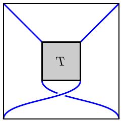
First, we may create a new tangle by changing all the undercrossings to overcrossings and vice-versa. Under this operation, the tangle $T$ becomes the tangle $-T$, which we will represent by shading the tangle box. This notation makes sense because $-[n] = [-n]$.
 |
|
 |
| $T$ |
|
$-T$ |
Next, we may rotate a tangle $T$ about a horizontal axis through the center of the ball to create a tangle $T^h$.
Similarly, we may rotate $T$ about a vertical axis to obtain $T^v$.
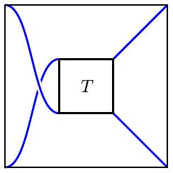
With this in mind, we see that $$ [\pm 1] + T \sim T^h + [\pm 1] $$
through an isotopy known as a horizontal flype.
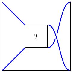
Similarly, a vertical flype shows that $$ [\pm 1] * T \sim T^v * [\pm 1] $$
With these tools in hand, we can now explain a rather surprising result:
$T^h \sim T$ and $T^v \sim T$.
To see why, notice that this result holds for $[0]$, $[\infty]$, $[1]$, and $[-1]$.
We now make the inductive assumption that the result holds for all tangles having $n$ crossings. Suppose that $T$ is a tangle having $n$ crossings, and consider $T+[1]$.
Applying a horizontal flip gives $(T+[1])^h \sim T^h + [1]$.
By the inductive assumption, $T^h\sim T$ so we have $(T+[1])^h\sim T + [1]$ as we hoped to find. There are, of course, several other cases to check, but they proceed in roughly similar ways.
Since we had earlier seen that $[\pm 1]+T\sim T^h+[\pm 1]$, we now have
$ \begin{align*} [\pm 1] + T & \sim T + [\pm 1] \\ [\pm 1] * T & \sim T * [\pm 1]. \\ \end{align*} $
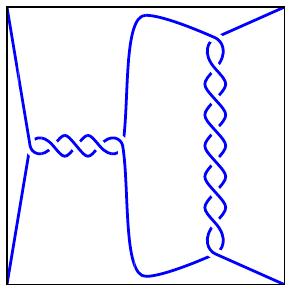
In this way, the rational tangle that we showed earlier in twist form may rewritten: $$ [5] + \left(\frac{1}{[2]} * \left([2] + \frac1{[3]} + [-2]\right) * \frac1{[3]}\right) \sim [5] + \frac1{[8]}. $$ as illustrated below:
 |
$\sim$ |
 |
This shows that we may generate all rational tangles by twisting the right endpoints and twisting the bottom endpoints. We may take this a little further by introducing another operation on tangles. Given a tangle $T$, the tangle $T^r$ is obtained by rotating the tangle box by $90^\circ$ in the counterclockwise direction.
|
 |
| $T$ |
$T^r$ |
Drawing a few pictures will convince you that $$ T * [-1] = (T^r + [1])^r. $$ A little more work shows that we can generate every rational tangle by applying to $[0]$ a sequence of addition and rotation operations:
$ \begin{align*} A: T & \mapsto T+[1] \\ R: T & \mapsto T^r. \\ \end{align*} $
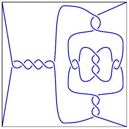
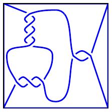
Here, for instance, is the rational tangle resulting from the sequence $AAARAAAARAA$.
Comments?
Tangle colorings and rational numbers
Conway showed that there is a one-to-one correspondence between rational tangles and rational numbers. Following Kauffman and Lambropoulou, we will describe this correspondence using tangle colorings.
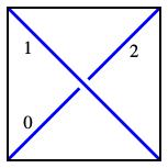
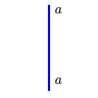
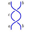
Given a tangle diagram, a tangle coloring is defined by labeling each arc with an integer such that at every crossing, as shown below, we have $a+b = 2c$.
For instance, the labeling below is a coloring.
It is easy enough to see that every tangle has a diagram that may be colored. To begin, the diagrams for the tangles $[0]$ and $[\infty]$ may be colored.
Performing the operation $A$, which means adding a twist on the right, adds one crossing and one arc with a free end. The coloring rule tells us how to label the added arc, as illustrated below. Similarly, applying the operation $R$ to a tangle with a coloring will produce a coloring on the resulting tangle.
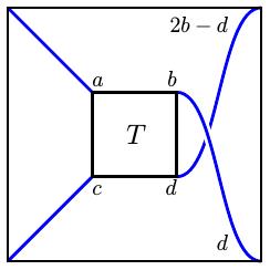
Given a coloring of a diagram for $T$,
the
color matrix will be the $2\times2$ matrix $$ \left[ \begin{array}{cc} a & b \\ c & d \\ \end{array} \right] $$ consisting of the labels on the four free ends. We will associate the rational number $$ f(T)=\frac{b-a}{b-d} $$ to the tangle $T$. Though it may not be immediately clear, this number completely characterizes the tangle.
For instance, the coloring of the tangle diagram $T$ above has the color matrix $$ \left[ \begin{array}{cc} 3 & 10 \\ 0 & 7 \\ \end{array} \right] $$ meaning that $f(T)=7/3$ is associated to that tangle.
It turns out that this rational number depends on neither the diagram of the tangle nor the coloring. This is explained by the following two facts.
- Given a coloring of one diagram of $T$, any other diagram has a coloring with the same coloring matrix.
This is because any two diagrams of the same tangle are related by a sequence of Reidemeister moves illustrated below.
| Move I: |
 |
$\longleftrightarrow$ |
 |
| Move II: |
 |
$\longleftrightarrow$ |
 |
| Move III: |
 |
$\longleftrightarrow$ |
 |
Given a coloring of a tangle diagram, any of the Reidemeister moves produces a coloring of the new diagram with the same color matrix. This is illustrated for the first two moves below; the third move is also easily checked.
| Move I: |
 |
$\longleftrightarrow$ |
 |
| Move II: |
 |
$\longleftrightarrow$ |
 |
- If one coloring of a diagram of $T$ has color matrix $$ \left[ \begin{array}{cc} a & b \\ c & d \\ \end{array} \right], $$ then any other coloring of that diagram has color matrix $$ \left[ \begin{array}{cc} ma+n & mb+n \\ mc+n & md+n \\ \end{array} \right]. $$
Consider any two arcs of the diagram. There is a unique affine transform $A(x) = mx+n$ that maps the labels in one of the colorings into the labels in the other coloring. By the linearity of the coloring rule, all other labels must also be related by this function.
We would like to determine how this rational number behaves under our operations $T\mapsto T+[1]$ and $T\mapsto T^r$. Let's first consider how the color matrices behave.
For any color matrix, it is useful to note that $a+d=b+c$. This is clearly true for the tangles $[0]$ and $[\infty]$. From what we have seen above, if this expression holds for $T$, then it also holds for $T+[1]$ and $T^r$. Therefore, it is true for all color matrices.
A simple calculation now shows that
$ \begin{align} f(T+[1]) & = f(T) + 1 \\ f(T^r) & = -\frac1{f(T)}. \end{align} $
Conway showed that $f$ is a one-to-one correspondence between the set of rational tangles and the set of rational numbers with $\infty$ appended.
Comments?
Square dancing and the Euclidean algorithm
Conway described a game that creates tangles and then untangles them using only the operations $A$ and $R$. Four players stand at the four corners of a square. There are two ropes, and each player holds one end of one rope. Initially, the ropes form the tangle $[0]$, and players are asked to create a tangle from a sequence of $A$ and $R$. They are then asked to untangle the tangle using only these operations.
Let's begin with a simple example: $T=[1]$. We wish to find a sequence of operations that takes the tangle back to $[0]$. If we apply $A$, we arrive at $[2]$, which takes us further away from our target. Instead, let's apply $R$ to obtain $[-1]$, and then $A$ to arrive at $[0]$. That is, if we want to untangle $[1]$, we should apply the sequence $RA$.
Shown below is the result of applying $RA$ to $[1]$, which clearly leads to the $[0]$ tangle.
What about if we start with $[2]$? The following sequence of steps works.
| Operation |
$f(T)$ |
| |
$2$ |
| $R$ |
$-1/2$ |
| $A$ |
$1/2$ |
| $R$ |
$-2$ |
| $A$ |
$-1$ |
| $A$ |
$0$ |
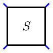
This shows that $RARAA$ will untangle $[2]$, which is shown in the smaller box below.
These examples illustrate the following algorithm to untangle a tangle $T$:
- If $f(T) \gt 0$, apply $R$ to obtain the new tangle $T$.
- If $f(T) \lt 0$, apply $A$ to obtain the new tangle $T$.
Let's see how this plays out with the rational tangle -17/7. We will write the rational numbers that appear in the form $p/q$.
| Operation |
$p$ |
$q$ |
| |
-17 |
7 |
| $A$ |
-10 |
7 |
| $A$ |
-3 |
7 |
| $A$ |
4 |
7 |
| $R$ |
-7 |
4 |
| $A$ |
-3 |
4 |
| $A$ |
1 |
4 |
| $R$ |
-4 |
1 |
| $A$ |
-3 |
1 |
| $A$ |
-2 |
1 |
| $A$ |
-1 |
1 |
| $A$ |
0 |
1 |
It is easy enough to prove directly that our algorithm will untangle the rational tangle $p/q$. However, we may achieve the same aim by noticing that our algorithm is simply a form of the Euclidean algorithm, which finds the greatest common divisor of a pair of integers $a$ and $b$.
The basis of the Euclidean algorithm is the observation that $$ \gcd(a, b) = \gcd(a-b, b). $$ If we assume $b>0$, we may write the algorithm as
- If $a \gt 0$, replace $a$ by $a-b$.
- If $a \lt 0$, replace $a$ by $b$ and $b$ by $-a$.
- If $a = 0$, then $b$ is the greatest common divisor.
For instance, if $a = 220$ and $b = 24$, we have
| $a$ |
$b$ |
| 220 |
24 |
| 196 |
24 |
| $\vdots$ |
$\vdots$ |
| -20 |
24 |
| 24 |
20 |
| 4 |
20 |
| -16 |
20 |
| 20 |
16 |
| $\vdots$ |
$\vdots$ |
| 0 |
4 |
Some readers may enjoy developing an algorithm that begins with a rational number $p/q$ and produces a sequence of $R$ and $A$ that forms the rational tangle corresponding to $p/q$ from $[0]$.
Summary
There is a much richer story lurking here. For instance, one may define yet another operation on tangles, callled inversion, which rotates the tangle and changes all over-crossings to under-crossings and vice-versa:
|
 |
| $T$ |
$\displaystyle\frac1T$ |
Following a line of thinking similar to that demonstrated above, Conway showed that every tangle $T$ may be written in a continued fraction form: $$ T \sim [a_1] + \cfrac1{[a_2] + \ldots \cfrac1{[a_{n-1}] + \cfrac1{[a_n]}}}. $$
The rational number associated to the tangle $T$ is then $$ f(T) = a_1 + \cfrac1{a_2 + \ldots \cfrac1{a_{n-1} + \cfrac1{a_n}}}. $$
Conway then used this description of tangles to develop a systematic notation for knots by decomposing them into sequences of tangles. In this way, he was able to create a list of all knots having 11 or fewer crossings. This list extended and corrected work of Tait, Little, and Kirkman from the late 1800's. Though Little took six years to compile his list, Conway, using his systematic description, completed his in an afternoon.
Interestingly, the study of knots grew out of Kelvin's attempt to describe the chemical elements as knotted vortex lines in the ether. In this way, he hoped to explain certain chemical properties of the elements as a result of this knottedness. Though this approach was eventually discarded, Tait was inspired to begin a study of knots, which in turn led to the mathematical theory of knots.
After roughly one hundred years of mathematical study, these ideas have found application in the modern study of DNA. Sumners provides some scale to the problem: if the nucleus of a cell were the size of a basketball, a DNA molecule would be roughly the size of a piece of fishing line stretching 200 kilometers. The recombination process is facilitated by the action of enzymes that allow one strand of the molecule to pass through another. The mathematical study of knots provides tools for describing this process. In particular, Goldman and Kauffman show how some of the ideas we have seen in this article may be used in this way.
Conway's square dance forms the basis of an engaging activity that one can conduct with, say, middle school students. It is hoped that this article helps to bridge the gap between the research literature and some descriptions of this activity published for teachers.
Comments?
References
-
John Conway. An Enumeration of Knots and Links, and Some of Their Algebraic Properties. Computational Problems in Abstract Algebra. Oxford, 329-358. 1970.
-
John Conway. Tangles, Bangles and Knots with John Conway. UC Berkeley Graduate Lectures. 2014
-
Louis Kauffman and Sofia Lambropoulou. Classifying and Applying Rational Knots and Rational Tangles, Contemporary Mathematics 304, 223-259. 2002.
-
Jay Goldman and Louis Kauffman. Rational Tangles, Advances in Applied Mathematics 18, 300-332. 1997.
-
Tom Davis. Conway's Rational Tangles.
Davis gives some ideas for using Conway's square dance with a group of middle or high school students.
-
DeWitt Sumners. Using Topology to Probe the Hidden Action of Enzymes. Notices of the American Mathematical Society 42 (5), 528-537. 1995.
-
C. Ernst and D.W. Sumners. A calculus for rational tangles: Applications to DNA recombination, Mathematical Proceedings of the Cambridge Philosophical Society 108, 489-515. 1990.
 David Austin