Multiplication Is Easier When It's Complex

Since multiplication represents repeated addition, it's natural that elementary students should learn addition before multiplication. But multiplication is also a significantly more involved operation. Let's look at the numbers p = 2642 and q = 5821 and compare the effort required to compute p + q and p·q using the algorithms that students are usually taught.

Both operations reduce the problem to some basic facts that need to be memorized: the addition and multiplication tables that show how to add and multiply pairs of single-digit numbers.

To add, we line the numbers up and add corresponding digits:

 

If we overlook the "carries," we see that adding two m-digit numbers requires us to perform m additions of single-digit numbers:

 

Multiplication is a bit different: we line the numbers up again, but now we multiply p by every digit in q.

 

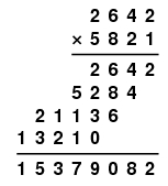
This means that we multiply every digit in p by every digit in q

 

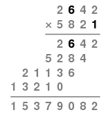
In this example, we must multiply 16 pairs of single-digit numbers compared to the 4 pairs of single-digit numbers added in the addition process. Generally speaking, adding two m-digit numbers requires m additions of single-digit numbers, while multiplication requires m² multiplications. This gives a quantitative expression to our experience that multiplication is a lengthier process than addition.

What happens if the numbers we want to multiply are very large, like these thousand-digit numbers?

p =

6133221551428429947549423892368426593568340909776595203443488845915534 8559816185847297968528018061504961949775198940315326035185896573238170 8583403808127741356506666602808101973537957581401397251417231569967460 7281227155082665645485738896664854336378985034734555175113749722286402 1691189467928013672198736815029442665248135623859274688398918797142052 2538339690326929935901293121901682980573701198387902489639283214237858 8273390332726110651403711317062781065355058879255875390455371705838971 968222402909247806471

and q =

3586426469517275960328285911560772141959079221744472281413773969376953 6955573024074572875488738605220715154637958999939573385032877419354873 3000715940899776840539293870100943601893809324233686808003377712741173 8893756867382264903704182677646777840519445822663403359978258586552601 7241934397819697570525857837806952474506321040345806117990125391058760 0055383364225656190420642997142800745223688058623621796382730846163591 9004988265659577082813442506200887524634184578054925915703746542585647 3815042424350970407428

There are, in fact, situations where we need to be able to work with numbers having millions of digits and perhaps more. For instance, certain encryption techniques used to protect information sent over the Internet rely on our ability to multiply large numbers. Also, a group of scientists has recently used techniques to multiply extremely large numbers (a press release states that these numbers, if written in hand, would stretch to the moon and back) to generate a huge list of so-called congruent numbers which has shed light on a very old problem in number theory (see the paper by Bradshaw et al in the references).

If p and q have millions of digits, multiplication would require trillions of single-digit multiplications. As the numbers grow large, the time required to multiply them using the traditional algorithm becomes prohibitively long. However, in this article, we'll describe a clever strategy for multiplying integers that takes a detour through complex numbers and that dramatically reduces the amount of work.

Multiplying integers is the same as multiplying polynomials

Let's look at our computation of p·q in a slightly different way. Remember what it means to consider an integer as a sequence of digits:

 

p = 2642 = 2 + 4·10¹ + 6·10² + 2·10³

so if we multiply p and q:

p·q	=	(2 + 4·101 + 6·102 + 2·103) × (1 + 2·101 + 8·102 + 5·103)
	=	(2 + 4·101 + 6·102 + 2·103) × 1
		+ (2 + 4·101 + 6·102 + 2·103) × 2·101
		+ (2 + 4·101 + 6·102 + 2·103) × 8·102
		+ (2 + 4·101 + 6·102 + 2·103) × 5·103
	=	(2 + 4·101 + 6·102 + 2·103)
		+ (4·101 + 8·102 + 12·103 + 4·104)
		+ (16·102 + 32·103 + 48·104 + 16·105)
		+ (10·103 + 20·104 + 30·105 + 10·106)
	=	2 + 8·101 + 30·102 + 56·103 + 72·104 + 46·105 + 10·106
	=	15379082

after collecting terms.

This feels a lot like multiplying polynomials. Indeed, if we use the digits of p and q to define polynomials

P(x)	=	2 + 4 x1 + 6 x2 + 2 x3
Q(x)	=	1 + 2 x1 + 8 x2 + 5 x3,

then we have p = P(10) and q = Q(10). Now define the polynomial R(x) = P(x)·Q(x) so that

 

R(x) = r₀ + r₁ x¹ + r₂ x² + r₃ x³ + r₄ x⁴ + r₅ x⁵ + r₆ x⁶

 

and r = R(10) = P(10) · Q(10) = p·q.

The seven coefficients of R(x) will give the digits of r, at least after we perform the "carry" operations we are sweeping under the rug. It is therefore our goal to find these coefficients. Of course, we could simply multiply the polynomials; however, that is equivalent to the computation we just performed with x replacing 10 and which requires 16 multiplications of pairs of single-digit numbers. We therefore have not saved any work.

We begin our search for a more efficient method with this crucial observation: the coefficients of a degree m - 1 polynomial are determined by the polynomial's values at m points. We will come back to the example considered above in a moment; however, let us work more generally for now. We will assume that r has m digits and that p and q have m/2. Since the degree of R(x) is m - 1, we will follow this outline:

1. Find the values of P and Q at m points, x₀, x₁, ..., x_{m - 1}.
2. Evaluate R at these points using the rule R(x_s) = P(x_s)·Q(x_s).
3. Use the values of R(x_s) to determine the coefficients r_t.

Notice that the second step only requires m multiplications; if m is large, this is much less than the roughly m² required in the usual algorithm. If we can find an efficient way to perform steps 1 and 3, we will therefore have found a faster way to multiply p and q. (In discussions like this, we will ignore the additions required since multiplication requires significantly more work.)

We may choose the points x_s however we please. For instance, an algorithm developed by Toom, and later refined by Cook, chooses the points to be x_s = s. We will see, however, that an elegant and efficient algorithm may be developed by choosing the points x_s to be roots of unity (roots of 1):

x_s = e^2πis/m.

We will begin by describing how to evaluate the polynomials P(x) and Q(x) at the points x_s.

Step 1: The Fourier Transform

We will assume that we have the polynomial

 

A(x) = a₀ + a₁ x + a_m-1 x^m-1 = Σ_t a_t x^t.

Let ω = e^2πi/m, a primitive m^th root of unity. We wish to evaluate A at the points x_s = ω^s so we will refer to these values as:

 

a_s = A(ω^s) = Σ_t a_t e^{2πi st/m}.

This process transforms the m coefficients a_t into m new values a_s by evaluating A at the points x_s. This is, in fact, a well-known transformation called the Discrete Fourier Transform and the values a_s are known as Fourier coefficients.

Evaluating one Fourier coefficient as a sum through the expression given above requires m multiplications. Since there are m Fourier coefficients, this would lead to m² multiplications, the same effort as our original multiplication algorithm. There is, however, a very efficient way, known as the Fast Fourier Transform, to find the Fourier coefficients, which we will now describe.

The Fast Fourier Transform

The Fast Fourier Transform provides an efficient means of computing the Fourier coefficients and is based on a rather simple observation. For reasons that will become apparent soon, we will assume that m, the number of coefficients a_t, is a power of 2. We then break the sum that defines the Fourier coefficient a_s into two smaller sums of even and odd values of t.

 

Notice that the two sums are themselves Fourier coefficients in transforms with half the number of terms; the first is the transform of the even terms a₀, a₂, ..., a_m-2, while the second is the transform of the odd terms a₁, a₃, ..., a_m-1.

Since the number of terms in these new transforms is now m/2, we may replace s in these sums by s', the remainder when s is divided by m/2.

We will denote the first sum as a_0|s' where the 0 in the subscript indicates we are using even terms. Think of this as representing the Fourier coefficient corresponding to s' when we transform the coefficients where t has a remainder of 0 when divided by 2.

In the same way, we will denote the Fourier coefficients of the transform of the odd terms by a_1|s'. Here again, think of the 1 in the subscript as telling us to consider indices t whose remainder, when divided by 2, is 1.

We may then rewrite our observation above as:

 

a_s = a_0|s' + ω^s a_1|s'.

The power of this observation lies in the fact that we may apply it again to compute the Fourier Transforms of the smaller sets. For instance,

 

a0|s'	=	a00|s'' + ω2s' a10|s''
a1|s'	=	a01|s'' + ω2s' a11|s''

where s'' is the remainder of s divided by m/4. Here, the subscript 00 indicates that we take the terms a_t where t has a remainder of 0 when divided by 4; likewise, 10 indicates the Fourier Transform of the terms whose indices have a remainder of 2 when divided by 4.

It will be helpful to express the indices t and s in binary form; that is, in the following, we will consider t and s to be strings of 0's and 1's. Our fundamental observation then becomes:

 

a_t|s = a_0t|s' + ω^2|t|s a_1t|s'.

In this expression, 0t is the result of appending a 0 to the left of the binary digits of t, |t| is the number of 0's and 1's in the string representing t, and s' is the new string of 0's and 1's formed by removing the left 0 or 1 from s.

If - represents the empty string, notice that

 

a-|s	=	as
and at|-	=	at.

Let's see how this works with an example. Suppose that m = 4 and the coefficients a_t are as follows:

 

t	0 = 00	1 = 01	2 = 10	3 = 11
at = at|-	3	7	1	4

Then we have ω = e^2πi/4 = i so that

 

a0|0	=	a00|- + a10|-	=	4
a0|1	=	a00|- - a10|-	=	2
a1|0	=	a01|- + a11|-	=	11
a1|1	=	a01|- - a11|-	=	3

With one more step, we find the Fourier coefficients a_s:

 

a0 = a-|00	=	a0|0 + a1|0	=	15
a1 = a-|01	=	a0|1 + i a1|1	=	2+3i
a2 = a-|10	=	a0|0 - a1|0	=	-7
a3 = a-|11	=	a0|1 - i a1|1	=	2-3i

To understand the amount of effort required in this process, let's reorganize the information into a table as shown below:

 

	00	01	10	11
at = a**|-	3	7	1	4
a*|*	4	2	11	3
as = a-|**	15	2+3i	-7	2-3i

At the top of the table are the coefficients a_t with which we begin while the bottom row contains the Fourier coefficients a_s that we seek. To generate an entry in an intermediate row requires one multiplication so each row requires m multiplications. The number of rows is lg(m), the base 2 logarithm of m. This means that generating the entire table takes m lg(m) multiplications. When m is large, this is significantly less than the m² multiplications required to find the Fourier coefficients by evaluating the polynomial A(x_s).

For instance, if m = 2²⁰, the number of multiplications required to perform the Fourier Transform through polynomial evaluation is 1099511627776, while the number required using the Fast Fourier Transform is 20971520. In other words, the Fast Fourier Transform reduces the amount of work by a factor of roughly 1/50,000.

Let's now return to our example where p = 2642 and q = 5821. We wish to find the product r = p·q.

Since p and q both have four digits, we expect that r will have less than eight digits. We need m to be a power of 2 so we take m = 8 and regard our polynomials as

 

P(x)	=	2 + 4 x1 + 6 x2 + 2 x3 + 0 x4 + 0 x5 + 0 x6 + 0 x7
Q(x)	=	1 + 2 x1 + 8 x2 + 5 x3 + 0 x4 + 0 x5 + 0 x6 + 0 x7.

To evaluate these polynomials at the points x_s = e^2πis/8, we will apply the Fast Fourier Transform with ω = e^2πi/8. Here are the steps required to find the Fourier coefficients p_s

 

	000	001	010	011	100	101	110	111
p***|	2	4	6	2	0	0	0	0
p**|*	2	2	4	4	6	6	2	2
p*|**	8	2+6i	-4	2-6i	6	4+2i	2	4-2i
p|***	14	2+6i+ω(4+2i)	-4+2i	2-6i-ω(4-2i)	2	2+6i-ω(4+2i)	-4-2i	2-6i+ω(4+2i)

This gives the Fourier coefficients p_s. In the same way, we may find the Fourier coefficients q_s. The results are summarized below.

 

s	0	1	2	3	4	5	6	7
ps	14	2+6i+ω(4+2i)	-4+2i	2-6i-ω(4-2i)	2	2+6i-ω(4+2i)	-4-2i	2-6i+ω(4+2i)
qs	16	1+8i+ω(2+5i)	-7-3i	1-8i-ω(2-5i)	2	1+8i-ω(2+5i)	-7+3i	1-8i+ω(2-5i)

Alert readers will notice that there is some symmetry in the sequence of Fourier coefficients stemming from the fact that the polynomial coefficients are real. This symmetry may be exploited to make the algorithm even more efficient.

Step 2: Convolution

Remember that the Fourier coefficients p_s and q_s, are found by evaluating the polynomials P and Q at the points x_s. We may therefore find the Fourier coefficients r_s = R(x_s) by simply multiplying p_s and q_s. That is,

 

r_s = p_s · q_s.

As will be mentioned later, this simple observation is an incredibly useful fact and one of the reasons the Fourier Transform is a ubiquitous tool in applied mathematics. We will therefore state it as a theorem. The process by which we compute the coefficients in a product of polynomials is known as convolution so we have the

 

Convolution Theorem: The Fourier coefficients of a polynomial R(x) = P(x) · Q(x) are obtained by multiplying the Fourier coefficients of P(x) and Q(x).

Applying the convolution theorem in our example, we find

 

s	0	1	2	3	4	5	6	7
ps	14	2+6i+ω(4+2i)	-4+2i	2-6i-ω(4-2i)	2	2+6i-ω(4+2i)	-4-2i	2-6i+ω(4+2i)
qs	16	1+8i+ω(2+5i)	-7-3i	1-8i-ω(2-5i)	2	1+8i-ω(2+5i)	-7+3i	1-8i+ω(2-5i)
rs	224	-70+20i+ω(-38+56i)	34-2i	-70-20i+ω(38+56i)	4	-70+20i+ω(38-56i)	34+2i	-70-20i+ω(-38-56i)

Notice that only m multiplications are needed in this step. In fact, we may think of this step as being analogous to the addition algorithm where we found p + q by adding corresponding digits of p and q. In the technique we are developing, we multiply p and q by multiplying their corresponding Fourier coefficients.

Step 3: Finding the coefficients of R(x)

The final step of our process--recovering the coefficients of the polynomial R(x) from the Fourier coefficients--is accomplished using the inverse Fourier Transform. It is straightforward to verify the following: if we construct a polynomial using the Fourier coefficients a_s,

 

A (x) = a₀ + a₁x + ... + a_m-1 x^m-1

then

 

a_t = A (ω^t) / m = 1/m Σ_s e^-2πist/m

where ω is the complex conjugate of ω. Notice that this expression is closely related to the Fourier Transform; we have simply replaced ω by its complex conjugate and, after the sum is evaluated, divided by m. We may therefore perform the inverse Fourier Transform using the Fast Fourier Transform with ω replaced by ω. This means that the inverse Fourier Transform may also be performed using m lg(m) multiplications.

Applying this to our example, we find the coefficients of R(x) as follows:

 

r0	r1	r2	r3	r4	r5	r6	r7
2	8	30	56	72	46	10	0

which again gives

 

r = 2 + 8·10 + 30·10² + 56·10³ + 72·10⁴ + 46·10⁵ + 10·10⁶ = 15379082

Summary

This technique, which is usually called Schönhage-Strassen multiplication in acknowledgment of its creators, represents a significant savings in effort. The traditional algorithm requires effort proportional to m² while Schönhage-Strassen reduces this to m lg(m). Since the logarithm lg(m) grows much more slowly than does m, Schönhage-Strassen is a superior algorithm when m is large.

In our discussion, the integers p and q have been represented in base 10, using digits 0 - 9. It is, of course, possible, and even desirable, to apply this technique using different bases. In particular, choosing a base that is a power of 2 is natural since we will be performing these computations on a computer that will represent the integers in binary form. A careful analysis of the algorithm reveals optimal values for the base.

The Fourier Transform is a fundamental tool in mathematics and its applications for it provides a means of understanding periodic phenomena. For example, it plays an important role in the theory of digital electronics and, in particular, digital music. However, it is the Fast Fourier Transform that enables this theory to be put into practice; the Schönhage-Strassen technique is, in fact, one that is much more widely applicable, in broad outline at least.

For instance, digital signals are frequently "filtered" by convolving the signal with another signal having specific characteristics. As we've seen, convolution is a computationally intensive task; however, the Fast Fourier Transform and the Convolution Theorem give a practical means of convolving signals by multiplying the Fourier coefficients of the signals.

In this way, the Fast Fourier Transform has played a fundamental role in the development of new communications technologies. Though this technique is often credited to a 1965 paper of Cooley and Tukey, the essential idea of the Fast Fourier Transform, computing Fourier coefficients through a recursive process, was used by Gauss in 1805 to calculate the orbit of the asteroid Pallas and has appeared in many forms over the past two centuries.

References

• Arnold Schönhage, Volken Strassen, Schnelle Multiplikation Großen Zahlen, Computing 7, 1971, 281-292.
  The original paper that describes the use of the Fast Fourier Transform for integer multiplication.
   
• Donald Knuth, The Art of Computer Programming, Volume 2: Seminumerical Algorithms, 3rd edition, Addison-Wesley, 1998.
  Knuth gives a careful analysis of the running time of this algorithm.
   
• William Press, Brian Flannery, Saul Teukolsky, William Vetterling, Numerical Recipes in C: The Art of Scientific Computing, 2nd edition, Cambridge University Press, 1992. Available online at www.nr.com.
  This reference gives an implementation of the Fast Fourier Transform and several variations.
   
• Michael Heideman, Don Johnson, and C. Sidney Burrus, Gauss and the history of the fast Fourier transform, IEEE ASSP Magazine 1 (4), 1984, 14-21.
   
• Andrei Toom, The complexity of a scheme of functional elements realizing the multiplication of integers, Soviet Mathematics Doklady 3, 1963, 714-716.
   
• Stephen Cook, On the minimum computation time of functions, Ph.D. thesis, Department of Mathematics, Harvard University, 1966.
   
• Robert Bradshaw, William Hart, David Harvey, Gonzalo Tornaria, Mark Watkins, Congruent number theta coefficients to 10¹², preprint available at www.warwick.ac.uk/~masfaw/congruent.pdf.
  This paper details recent progress in generating large numbers of congruent numbers using ideas related to Schönhage-Strassen multiplication. A press release, A Trillion Triangles, from the American Institute of Mathematics gives a non-technical description.