The Mathematics of Surveying: Part II. The Planimeter
Posted June 2008.
The second of two columns on the mathematics of surveying (the first is here). ...
Bill Casselman
University of British Columbia, Vancouver, Canada
cass at math.ubc.ca
John Eggers
University of California, San Diego
jeggers at ucsd.edu
A planimeter is a table-top instrument for measuring areas, usually the areas of irregular regions on a map or photograph. They were once common, but have now largely been replaced by digital tools.
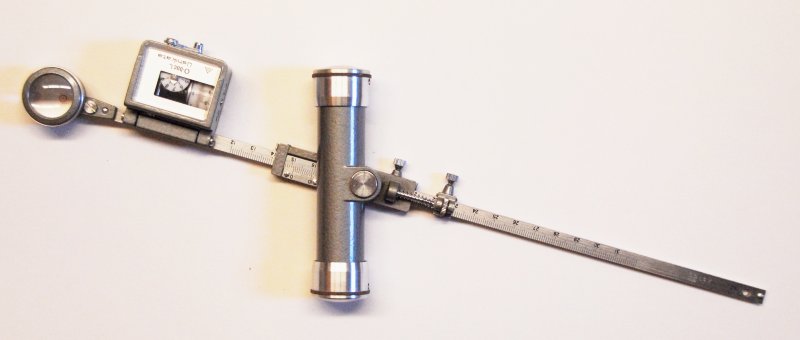
The following picture gives some idea of the setup. The pole arm rotates freely around the pole, which is fixed on the table. The tracer arm rotates around the pivot, which is where it joins the polar arm. You trace a curve in the clockwise direction with the tracer, and as you do so the measuring wheel rolls along, and the total distance it rolls is accumulated on the dial. The support wheel keeps the thing from flopping over. At the end, you read off a number from the dial, and after multiplication by a factor depending only on the particular configuration of the planimeter, you get the area inside the curve.

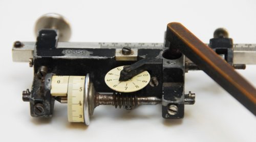
The next figure gives you a better view of the mechanism.

We call the carriage the assembly of wheels, dial, and pivot. In the next picture you get a better look at it, and can see the worm drive that causes the dial to rotate as the measuring wheel moves.
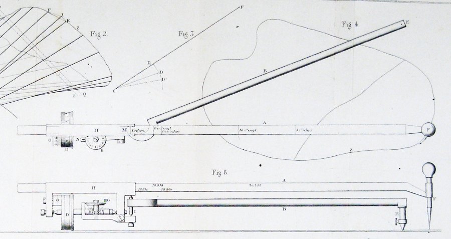
Here is the diagram of the original planimeter, from the article by Jakob Amsler that introduced it:
How can such a simple thing measure areas?
Geometry of the planimeter
The clockwise movement of the planimeter is the direction opposite to what mathematicians have decided should be positive rotation. Rather than violate this convention, we are going to work from now on with a mathematician's planimeter, in which you move counter-clockwise. Like other mathematicians' fantasies, there are none on the planet!
There are some restrictions on how to place the planimeter with respect to the curve you want to trace. The carriage can be slid along the tracer arm, but in all cases the length l of the tracer arm is less than that the length r of the pole arm. This means that the tracer can never get within a distance r - l of the pole. On the other hand, when it is fully extended, the tracer can never reach beyond r + l. So the curve to be traced must lie within the annulus between two circles, one with radius r - l, the other r + l.

In fact, it should become clear in a moment that the arms should never be completely extended, so the curve to be traced must lie completely inside the annulus. Furthermore, normally the pole is placed on the outside of the curve.

For a given point in the annulus there are exactly two possible configurations of the planimeter that place the tracer on that point. Choosing one point or the other means choosing a sign for a square root. We call this choosing an orientation for the planimeter. It is positive if the square root is positive. Once an orientation has been chosen, it will remain the same unless the arm is fully extended. This must never happen. As long as your curve is entirely within the annulus, the configurations of the planimeter will vary smoothly and uniquely with the path of the tracer.
The next thing to do is to understand a few things about the motion of the measuring wheel. As the following picture shows, if the wheel travels in a straight line a distance C, the wheel rotates through an angle θ = C/R where R is its radius.

So it is really true that the rotation of the wheel and the distance traveled by the tracer arm have some relationship to each other. But this relationship is a bit subtle. If the arm just moves straight ahead a distance C, the area swept out will be lC, but if it shifts parallel to itself the area swept out will be 0. In the first case, a point on the circumference of the wheel will move distance C. In the second case, the wheel will not move at all. And if the arm translates obliquely, the wheel will rotate a distance equal to the altitude of the parallelogram covered by the arm. In all cases where the arm translates parallel to itself, the area swept out by the portion of the tracer arm between the pivot and the tracer will be equal to lC, where C is the distance measured by the rotation of the wheel. This is the basic fact relating the arm's motion to the motion of the measuring wheel.

The way to phrase this precisely is that no matter how the the arm moves, the distance measured by the wheel is the path integral

where Γ is the path traveled by the point of the arm where the measuring wheel is attached, n is the unit vector perpendicular to the arm at any moment, and t is the unit vector pointing in the direction of travel (so that, for example, if the arm is moving parallel to itself the dot product of n and t is 0).
Guldin's Theorem
Next we are going to try to make the behaviour of the planimeter intuitively clear, but first we are going to look at a special kind of planimeter, and in this case prove a more general result. Suppose we take a single freely moving arm of length l and attach to it a measuring wheel of radius R right in its center.

Then we move the arm around on the plane. If the measuring wheel rotates through a total angle of θ radians as the arm moves around, the distance a point on the circumference travels is C = θR.
Guldin's Theorem. In this situation, the total area swept out by the arm is the product lC.
Area here is interpreted with a sign. If the arm just rotates around its center, one half of the arm goes forward and the other backward, and the two cancel.
We have already seen that Guldin's assertion is valid in the case the arm just translates. Of course this doesn't always happen - the arm may rotate as it moves as well as translate. But we can see what is happening by chopping up the swept area as follows:
Because the measuring wheel is in the center of the arm, as the arm rotates, it squishes the little blocks on one side as it expands them on the other. These effects cancel each other out exactly.
A completely rigorous proof can be given by using the formula for change of variables in a double integral and the expression for wheel travel as a path integral.
Now suppose the wheel is placed somewhere else. Say its position is c + v where c is the center of the arm, and v a vector along the arm. The length of v will remain fixed, say at ρ. The path that the wheel follows is c(t) + v(t). The path integral is now

The first integral is the distance the wheel would travel if it were at the center of the arm. In the second, the vector v(t) is always perpendicular to n, and v(t) has constant length. The vector v(t) moves around on a circle of radius equal to ρ. Therefore the dot product of n and v'(t) is just the signed length of v'(t), and the second integral is equal to ρ times the total rotation of the arm. Hence:
If the wheel is at distance ρ from the center of the arm, the distance C the wheel measures is C0 , the distance that would be measured if the wheel were at the center, plus ρ times the total angle θ that the arm rotates.
You can see immediately one simple case of this by rotating the arm around its center. Combining this with Guldin's Theorem, we see that in all cases:
C = C0 + ρ θ
Area swept out = l C0 = l C - l ρ θ
The full result
Guldin's Formula gives a signed area - if you sweep backwards over an area, the wheel goes backwards and you cancel area you have already covered. If we apply this to the case where the free arm comes back exactly to where it started, we see that lC is equal to the area of the closed region traced out by the right end of the arm minus that of the region swept out by the left one.

In the case of the polar planimeter, the bottom of the arm is restricted to an arc of the circle of radius r with center at the pole, hence l C is the area traced out by the tracer. Furthermore, normally the pole lies outside the region to be measured, and in this case the total amount of rotation of the arm has to be 0. So in this case we have
Area of the region traced = lC
Here is the figure included by Jakob Amsler, the inventor, in his original paper on the instrument he invented:
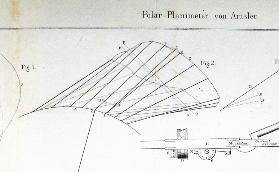
It seems pretty clear from this that Amsler derived his construction through some form of Guldin's theorem.
Planimeters and Green's Theorem
As we have already mentioned, having chosen the orientation of the planimeter, the planimeter configuration is a continuous function of the tracer position. Say we choose the positive orientation. Then we can attach to each point of the annulus a unit vector n, the one pointing counter-clockwise and perpendicular to the tracer arm at the tracer.
How the measuring wheel is going to respond to motion along the curve in the next instant depends on the angle between this vector and the unit tangent vector of the curve. At A in the picture above, the measuring wheel is not going to move because the motion along the curve is parallel to the tracer arm. At B if the tracer moves a small distance ds, so will the measuring wheel. And at C the measuring wheel will move some distance in between 0 and ds. To be precise, suppose t is the unit tangent vector at some point of the curve. If the tracer moves distance ds along the curve, at that point the measuring wheel will move a distance d ds, where d = n . t, the dot product of the unit vectors t and n. In other words, if we move all around the curve Γ the measuring wheel will move a total distance equal to the integral of n . t ds (dot product), or
But since every point of the annulus corresponds to a unique positive configuration of the planimeter, we can assign a vector n to every interior point of the annulus, and it therefore defines a vector field. The curve Γ is the boundary of its interior Ω, and by one of our assumptions this is contained entirely in the region where n is defined. Green's Theorem tells us that the path integral around the boundary of this region is also equal to a certain integral over Ω: Therefore
More precisely, Green's Theorem tell us that

where n = [p,q] is the vector field involved. The integrand in the double integral is called the curl of the vector field.
This doesn't seem to get us very far. What ought to happen is that the curl is a constant 1. In principle, we could find a formula for the vector field n and calculate its curl, but that isn't very enlightening. We can take advantage of another fact, however. The vector field has circular symmetry, which means that it is determined by what it is on one radius. The cosine law gives us a simple formula for the circumferential component.
It follows from simple geometry in this figure that the circumferential component of n is
f(ρ) = cos(γ) = (ρ 2 + l 2 - r 2)/(2 ρ l)
The real point of Green's Theorem is that in order to verify that the integrand is 1 it suffices to verify that the path integral around suitable small paths is the same as the area. For this, we choose our regions to be as here:
Then l times the path integral is
l (ρ+dρ)( f(ρ+dρ)- f(ρ) ) dθ
or
(θ/2) ( (ρ + dρ) 2 - ρ 2)
which is the area of the region Ω.
Other kinds of planimeters
Guldin's Theorem implies that the motion of a measuring wheel will tell you the area traced out by the tracer whenever the arm with a measuring wheel on it traces out a curve but has one end restricted to a one-dimensional curve. This happens, for example, with the rolling planimeter, in which the pivot is restricted to a straight line by being on a rolling cylinder.
To find out more
 still makes and sells planimeters.
- Differential and Integral Calculus Volume II, R. Courant, Blackie & Son, 1936. The section on Guldin's Formula (pp. 294-298) offers an explanation of how the planimeter works.
- Amsler's original article, Vierteljahresschrift der Naturforschenden Gesellschaft in Zuerich, 1856. This is missing the diagrams, but they are here:
Our thanks to Donna Sammis of the Stony Brook University Library for locating the article and to her husband Robert for supplying photographs of the figures.
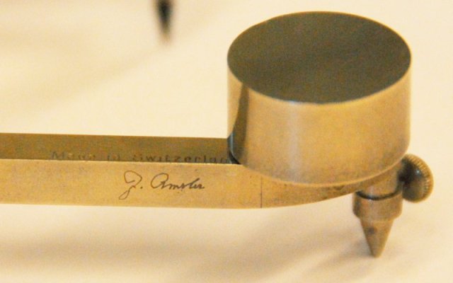
The company that Amsler founded produced instruments well into the 20th century. This photograph shows the logo, on a pantograph version of the planimeter:
- "About Planimeters," EngineerSupply. The company has also posted a video on YouTube.
Bill Casselman
University of British Columbia, Vancouver, Canada
cass at math.ubc.ca
John Eggers
University of California, San Diego
jeggers at ucsd.edu
Those who can access JSTOR can find some of the papers mentioned above there. For those with access, the American Mathematical Society's MathSciNet can be used to get additional bibliographic information and reviews of some these materials. Some of the items above can be accessed via the ACM Portal , which also provides bibliographic services.


