Keep on Trucking

Posted January 2010.

Joseph Malkevitch
York College (CUNY)
malkevitch at york.cuny.edu

Introduction

Love may make the world go round but what makes our daily lives so much easier is trucks. Trucks deliver the food that we eat to the supermarkets and restaurants we use, they deliver the gasoline to the stations where we refill the gas tanks in our cars, and they are responsible for a huge part of the movement of supplies throughout local regions and nationally.

And what helps make it possible for trucks to carry out all the deliveries they do is mathematics.

(Photo courtesy of Wikipedia)

Background

During World War II the Allies discovered that wars were not only waged by soldiers but by the people who designed the efficiency of the scheduling of troop movements and materiel that were necessary for soldiers to fight the war. With no lines of supply, soldiers can not be very effective. The ideas laid down during the war became codified in the area of knowledge that has come to be called operations research or management science. Operations research drew heavily on the mathematics and the nascent computer science to assist businesses, governments, and individuals in organizing their work (and play) more efficiently.

One early triumph of the newly emerging area of operations research was the codification of the linear programming model. Linear programming has been one of the most successful applied mathematical tools in history. It makes possible a wide array of scheduling, allocation and blending problems to be solved. Basically, the idea behind linear programming is to find the maximum or minimum value of a linear function (typically of many variables) where the variables are constrained by a system of linear inequalities. As computers have become faster, it is often possible to solve many large linear programming problems in real time. The best known algorithm for linear programming, pioneered by George Dantzig, is called the simplex method.

(George Dantzig)

Although the simplex method can in the worst case require exponential time to carry out, it runs very well in practice, a phenomenon which mathematicians are trying to understand better. There are polynomial-time algorithms for linear programming due to Leonid Kachiyan and Narendra Karmarkar. However, in many situations where linear programming is employed, the simplex method outperforms those polynomial-time algorithms, which fall into groups classified as interior point methods or ellipsoidal methods.

In many situations which one might like to model using linear programming, the values of the variables are restricted to non-negative integers. This extension of the linear programming model is known as integer programming. At the current time there are no known polynomial-time algorithms for integer programming, though there are special kinds of integer programming problems for which polynomial-time algorithms are known.

What has made linear programming so powerful is that the model is flexible enough to formulate a huge range of situations that come up in applied situations. Thus, linear and integer programming have found use in mixture problems, allocation of resources, blending questions (oils to make gasoline and meats to make cold cuts), and scheduling, to mention but a few. Many vehicle routing problems can be formulated in terms of linear and integer programming.

Here is the what the authors (G. Dantzig and J.H. Ramser of what was probably the first paper on vehicle routing from a mathematical perspective) wrote as the abstract to their paper:

The paper is concerned with the optimum routing of a fleet of gasoline delivery trucks between a bulk terminal and a large number of service stations supplied by the terminal. The shortest routes between any two points in the system are given and a demand for one or several products is specified for a number of stations within the distribution system. It is desired to find a way to assign stations to trucks in such a manner that station demands are satisfied and total mileage covered by the fleet is a minimum. A procedure based on a linear programming formulation is given for obtaining a near optimal solution. The calculations may be readily performed by hand or by an automatic digital computing machine. No practical applications of the method have been made as yet. A number of trial problems have been calculated, however.

Time has seen to it that ideas of this kind are being applied regularly, at the same time as the problem nurtures an ever growing collection of specialized applied and theoretical studies of mathematical models suggested by the original.

Some history

The first scholarly paper which addresses what today is called the vehicle routing problem (VRP) appeared in 1959 in the journal Management Science, whose first volume appeared only 4 years before in 1955. The authors of this paper were George Dantzig (1919-2005) and J. H. Ramser. Their work was also presented at the Fifth World Petroleum Congress held in New York in 1959. Dantzig was a well known and important figure in linear programming and operations research and was working for the Rand Corporation at the time. I was unable to find out much information about Ramser, whose full name was John Ramser. At the time he worked with Dantzig on this paper he was an employee of the Atlantic Refining Company in Philadelphia, which later became ARCO and was eventually absorbed into British Petroleum. He wrote at least one other quite mathematical paper ("Theory of Thermal Diffusion under Linear Fluid Shear") and was the author of a variety of patents. Ramser also played a role in the early development of SIAM (the Society for Industrial and Applied Mathematics), having served in its earliest days (1953-1956) on its governing council.

A few years after the Dantzig-Ramser paper another important milestone paper appeared. This paper by G. Clarke and J. W. Wright appeared in 1964. Clarke and Wright specifically discuss the work of Dantzig and Ramser but develop a rather different approach which has proved extremely fruitful. I know relatively little about Clarke and Wright. Clarke was affiliated with the Wholesale Cooperative Society of Manchester, while Wright worked at the University of Manchester (England). Their work will be treated later, but first let us look at a problem that actually predates the one formulated by Dantzig and Ramser (and which they mention in their paper) and which has had great importance of its own.

A special vehicle routing problem

Anyone sitting in traffic in a large city knows that trucks come in a staggering array of types, ranging from relatively small delivery trucks to the giant trucks that carry ore from mines to other locations. We will see that there are different types of problems that arise for these different types of trucks. Although there are many applied questions which involve trucks and, more generally, vehicles, what has come to be called the vehicle routing question has a special structure. Generally speaking, the goal of the problem is to minimize the cost of carrying out the needed work while not violating the constraints that may be imposed (e.g. truck capacity or the delivery at site 3 must be made between 2 and 3 p.m.). In particular, there is a very special case of the vehicle routing problem which is much better known than the vehicle routing problem itself. Known as the Traveling Salesman Problem, it first began to be studied in about 1930. This problem is so significant that there are whole books devoted only to issues related to the Traveling Salesman Problem (TSP).

Here is a "vanilla" formulation of the TSP which suggest how it got its name. A salesperson lives in X and must visit a finite number of locales A, B, C, ...,Z once and only once and then return to X, his/her home site. There is a cost of getting from home to any of the locales and a cost of getting between any pair of the locales. Find a tour for the salesperson that minimizes the cost of such a tour. How does one measure cost in such a situation? The cost may be time, distance, the cost of gasoline if the trip is by auto, the cost of train tickets if the trip is by train, etc.

The goal of solving a TSP is both to know what the minimal cost would be and to find the tour that achieves this minimal cost. The answer to a TSP in a particular case will depend on the costs associated with the "trips" between pairs of locations. The driving tour may be different from the airline tour. Furthermore, as is often the case when problems from the "real world" are examined within the mathematical world, one quickly sees that one has to make simplifying assumptions (this process is called mathematical modeling) to analyze what is happening. For example, whereas when one thinks of distance it is natural to feel that the distance from U to V should be the same as the distance from V to U, and this would be true of Euclidean distance (or taxicab distance), in many applied situations like the TSP this assumption that distance is "symmetric" will not hold. For example when one drives from U to V in a city, it would be rare, because there are one-way streets, that the distance from U to V will be the same as the distance between V and U. Thus, already the formulation of the TSP given above is "too simple" for some situations. In some cases two costs between sites would be needed: the cost of going from U to V and a different cost going from V to U.

One traditional way to model a TSP is to use the geometric tool consisting of dots and line segments called a graph. Home (or the depot) and the sites to be visited are represented by dots known as vertices, and two sites are joined by an edge if there is a finite cost to get between the two sites. If the cost involved in going from U to V is not the same as the cost in going from V to U, one uses a directed graph instead of a graph, the difference being that in a directed graph there are line segments with arrows on them. Typically in the undirected case the graph one gets is a complete graph, meaning that there is an edge between every pair of vertices. Each edge is also assigned a weight which gives the cost between the sites it joins.

Ordinary Euclidean distance also has the property that the distance from U to V plus the distance from V to W is greater than or equal to the distance between U and W. When this situation holds for all triples of sites U, V, and W we say the triangle inequality holds. The triangle inequality is one of the usual "axioms" (rules) that mathematicians assume an "abstract" distance obeys. However, for driving distance this may not be true because roads may not follow Euclidean distance. Thus, due to mountainous terrain it may be that the distance to drive from U to W directly may be longer than going from U to V and then from V to W. So the "costs" that are mentioned in the TSP may or may not obey the triangle inequality. Another property of distance is that the distance between U and V is either a positive number or zero. In fact, it will be zero in the situation for an abstract distance if and only if U and V are the same site. However, it is convenient in the applications to which the TSP is applied to allow the cost from U to V to be negative. One can interpret this negative cost as a subsidy for going from U to V. Figure 1 has symmetric distances (distance from U to V equals the distance from V to U) but has subsidized edges AC and XB. In other examples we might have a different distance from U to V than from V to U. Also we might have a positive cost from site M to N but a negative cost from N to M. The evolution of the TSP has followed the course of many mathematics problems. Initially inspired by a practical and intuitive problem in operations research, it not only became important to solve the problem for these practical reasons but it was quickly realized that ideas related to solving this problem had important aspects for mathematics itself. As a consequence, many variants of the problem emerged which had intrinsic interest as mathematics problems, but these in turn represented results which had applicability of their own.

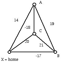
Diagram of a four city TSP with subsidized edges

Figure 1 (4-site instance of a TSP, with edge subsidies)

One of the amazing things about important mathematical problems is how they pop up in places one might not initially think of. For a long time my favorite unexpected application of the TSP was to the fabrication of chips. To manufacture a chip requires the insertion of various components, typically using a robot. The optimal insertion order for these insertions involves solving an asymmetric TSP. However, I recently learned from David Johnson of work by Adam Buchsbaum (and colleagues). The basic idea is that large companies such as a phone company generate tables of information consisting of many fixed length records. A large company might have to store over a billion records per month, where the records could contain such information as the exchanges between which calls are made, call lengths, and costs, etc. In light of the huge amounts of data involved, it is desirable to store this data in compressed form. While for photos that appear in articles such as this one, compression that loses information is acceptable, for the application in this case lossless compression is mandatory. Oversimplifying greatly, it turns out that one can compress parts of the data set (sets of columns) and follow this by a compression of additional columns that make up the data set. The space used up at the end will generally depend on the order in which the sequence of compressions is carried out as well as the ordering of the columns in the group being compressed. Hence, one can profitably use the TSP (the asymmetric case) as one piece in the methodology to store the large data set as compactly as possible.

How hard is it to solve vehicle routing problems? Not surprisingly, the amount of "work" necessary to solve a problem by hand or using a computer increases dramatically as the number of sites to be visited grows and the complexity of the constraints to be dealt with increases. So a decision has to be made as to how much "money" (e.g. time and effort) to spend in finding an exact (optimal) solution versus an approximate solution which is known to be not far from an optimal solution, or one may be willing to settle for a solution which "works" (e.g. meets the constraints) and which can be obtained without undue effort. For example, in scheduling a collection of vehicles to deliver meals on wheels to elderly or ill people in a city, it might not make sense to spend lots of extra money to find a solution that is 3% better than one that can be found easily because the elderly can pass away or enter the hospital for a few days and not require a food delivery. Thus, the routes designed on a given day perhaps will have to be different from those on the next day. Hence, for this situation one needs an algorithm which finds an answer quickly and has the flexibility to handle sites that will enter or drop out of the collection of locations where a "delivery" must be made. On the other hand, if one is delivering things to supermarkets or to gasoline stations, it may well be worth spending the extra time and effort to find a 3 percent better solution than the one currently used because over a period of time in using the less costly solution one can compensate for the costs that getting the better solution entails. So one of the considerations for both the TSP and more general vehicle routing problems is that of finding an exactly optimal or approximately optimal solution. However, as problems grow larger, the amount of work can be expected to grow whether or not one wants an exact or approximate solution.

The branch of mathematics and computer science known as complexity theory address the questions of how much "work" it takes to solve various kinds of problems using an algorithm designed to run either on a sequential or parallel computer. The basic idea is that there is a number n associated with the different instances of the problem which measures the size of the problem. For example, for the TSP the number n is usually the number of sites to be visited. As n grows larger for the TSP, what is the mathematical function that describes the amount of work necessary to solve the problem?

When problems of size n can be solved using an algorithm that uses an amount of work that grows as a polynomial in n (even if the degree of this polynomial is large), the algorithm for the problem is considered a (relatively) easy one. However, when any algorithm to solve a problem uses an amount of work which grows faster than an exponential function of n, the problem is considered hard. The collection of NP-complete problems are problems for which no known polynomial-time algorithm exists but for which it has not been proved that an exponential-time algorithm is required. Furthermore, if any problem in this collection could be shown to be solvable in polynomial time or require exponential time, all the problems in the collection would have the same status with regard to their difficulty. Thus, NP-complete problems are all computational "hard" or all computationally "easy" but we don't know which! The general version of the TSP was shown to be NP-complete as early as 1972 by Richard Karp. Many variants of the TSP have been shown to be NP-complete. Some good news is that the Euclidean distance version of the TSP admits a polynomial-time approximation method. However, nearly all variants of the VRP are "at least as hard" as the TSP and, thus, for reasonably large problems, exact methods may not be practical. This suggests using heuristic methods: Algorithms that are not guaranteed to be optimal but can be implemented efficiently even for relatively large problems.

The Clarke-Wright heuristic

One seminal paper in the area of vehicle routing was published in 1964 by G. Clarke and J.W. Wright and has come to be known as the Clarke-Wright Algorithm. The Clarke-Wright Algorithm is a "greedy" algorithm which has a very intuitive structure.

As in many applied situations, we construct a mathematical model (simplified view) of what we want to study, and if this leads to some success in obtaining insight, we will expand the model to more "realistic" settings.

Here is the basic situation that the Clarke-Wright method addresses: A collection of identical trucks, in which each truck has a fixed amount of capacity--typically measured in how much weight (in some cases volume) it can carry--is located at a single site called the depot. There is a collection of customers to whom deliveries must be made from the depot. The size of the delivery might be different from one customer to the next or it might be the same for all customers. What is available is information about the distance or time between the depot and the sites as well as the same information between the sites. In some situations the time or distance between two locations may not be the same in both directions. Thus, as part of the problem specification it is important to make sure whether symmetric or unsymmetric distances are being used.

Let us consider a specific example to give the flavor of what is involved and to help you think about what is going on. You can then see how some simple intuitive ideas can be used to get insight into problems of this kind.

We will assign the depot from which the one or more vehicles are to be dispatched the name "0" and all the other sides will be numbered from 1 to n. The cost of a trip between two sites i and j (one of which may be the depot) will be denoted c_i,j. Thus, for example, c_2,3 will denote the cost of going from site 2 to site 3 while c_4,0 will denote the cost of going from site 4 to the depot. We will, only for convenience, assume that the cost of going from i to j is the same as going from j to i. Now if we currently have a vehicle that goes from the depot to i and back and another vehicle going from the depot to j and back, the cost for the first vehicle will be c_0,i + c_i,0 which, since these two costs are the same, is 2c_0,i, and, similarly, we get a cost of 2c_0,j for the second vehicle to go from the depot to j and back. If it is possible to use one truck for both of these "deliveries" we can consider the route which "merges" these two "subroutes" and go from the depot to i and then continue on from i to j (rather than going back to the depot) and then return to the depot from j.

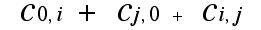
Now the cost of the trip from the depot to i, then to j, and then to the depot is:

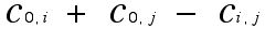
so if we replace the two trips from the depot to and from each of i and j by the trip from the depot to i and then to j and then back to the depot, we can compute the different in cost between these two different routings:

The number just computed is the "savings" obtained when the tours that go from the depot to i and the depot to j are "coalesced." (From different points of view one can think of this merging process as taking two separate routes carried out by one vehicle as being collapsed to one tour for that truck or as two trips that are carried out by different vehicles now being carried out by a single vehicle.)

The Clarke-Wright heuristic algorithm is a "greedy" algorithm. This means that at each stage when something is carried out, a "locally" (at that moment) best decision is made. Of course, there is no guarantee that such locally good choices end up with a solution that is globally good or even nearly good. (For many greedy algorithms an optimal answer will be obtained.) There are by now many, many variants of the Clarke-Wright heuristic. I will try to give you the gist of the ideas in as non-technical language and notation as possible.

Begin by visiting the required sites by going from the depot to that site and back again. For a depot and 2 sites this will be represented by the single edges as in Figure 2. Now, if when we get to i from 0 (the depot) we go to j rather than going back to the depot immediately, and now return to the depot from j, it seems intuitively clear that we should save "cost." As we saw above, the saving in this case will be S_i,j as computed above. This savings will be positive when the costs obey the triangle inequality. So it would seem to be helpful to know how large the different savings will be between pairs of sites i and j. We can then try to adopt a "greedy" approach by trying to coalesce subtours at each stage using a "short cut" edge with the greatest savings (as suggested by the approach in Figure 2, where one can also think of the single edges as subtours, and not necessarily as a single edge).

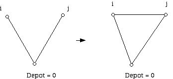Figure 2

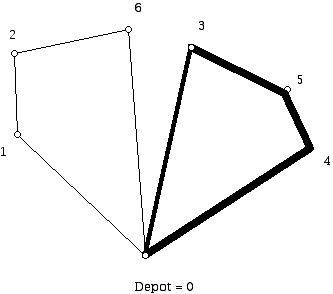
So the idea behind Clarke-Wright is to merge "subtours" when possible to get a longer, cheaper tour of all the sites. Figures 3 and Figure 4 show what subtours might look like when solving a moderately sized problem by hand. Note that if we have two trucks these diagrams might (depending on the constraints of the problem) represent the final result of the algorithm. However, when we are using the Clarke-Wright heuristic to solve a TSP we would not be finished at this stage. Using Figure 4 we can see the ways that these tours (which currently are: 0, 1, 2, 6, 0 and 0, 4, 5, 3, 0 listed in order, although they could be written in reverse cyclic order) might be merged. To merge these two circuits we could use edge 63 to get the circuit 0,1,2,6,3,5,4,0; edge 64 to get 01264530; edge 31 to get 04531260; or edge 41 to get 03541260 (or these four circuits in reverse cyclic order).

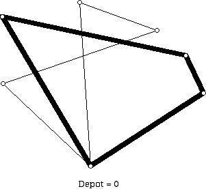Figure 3

Two tours which visually only share the depot

Figure 4

We will think of each of the two variants of the Clarke-Wright heuristic under consideration as having two steps. Step 1 is the same for both variants.

Step 1:

Compute the saving S_i,j associated with the edge i, j (i, j different and neither 0). Now order these savings in nonincreasing order.

Variant A:

Step 2

Begin with the edge at the top of the saving list.

Move through the list of savings. When considering the saving S_i,j check if there are currently tours using edges 0,j and 0,i and if these tours can be feasibly merged, do so by adding i,j to the tour and deleting edges 0,j and 0,i.

(Note: If the trucks being used for these two tours have limited capacity, one reason why it might not be feasible to join the two tours using edge i,j, even if the edge conditions above are met, is that the sizes of the pickups at i and or j, when added to the vehicle's load in this merged tour would exceed the room available on either truck being used for the smaller tours. One tries to merge tours as one goes through the list of savings. When one achieves a single tour for all the sites or runs out of edges, one terminates.)

Variant B:

Step 2

Begin with the edge at the top of the savings list.

Use the next edge in the savings list to expand the current route by using this edge to extend the tour currently being worked on. If this tour cannot be extended, try to extend another tour using this edge. If no tour can be extended using the current edge, move to the next edge in the savings list.

(Note: Initially, one can always add the maximum saving edge unless the capacity of the vehicles serving the sites at its ends are too large for one of the vehicles to be used. The idea here is to try to expand the current tour as long as possible with the edge providing the largest possible saving. One only moves on to another tour when the current tour cannot be added to.)

When there are other constraints such as capacity of vehicles or restrictions on the number of sites on a tour, etc., the algorithm above is modified to check that adding the edge i, j which has the greatest saving at a particular stage is feasible with respect to the constraints, in addition to being possible from the point of view of enabling the merging of the tours.

Experiments have been done to compare the two variants described above. There are some indications that Variant A tends to work better.

To give you the flavor of the Clarke-Wright algorithm we will discuss how to use Variant 1 to solve a very small example. In the graph below we have a depot, labeled 0, and four sites labeled 1 to 4. This example involves a complete graph on 5 vertices (every pair of the vertices is joined by an edge). Furthermore, there is a cost associated with every edge in the graph which you can interpret as the amount of time it typically takes to travel between the pair of sites that are at the ends of the edges.

Figure 5 (A four site instance of a VRP)

In this example, the driving times in each direction between two sites are the same. We also have the property that for of any three vertices the sum the lengths of any two sides of the triangle they form has weight greater than the weight (cost) of the third side. We will initially think of this as a TSP problem, that is, we want to find a reasonably short route from the depot which visits each site exactly once and returns to the depot. We initialize our solution by thinking of the vehicle going from the depot to each site and back again. At this stage we have the diagram in Figure 6. We will then see how to improve this very inefficient "tour" to one which hopefully would be a lot better.

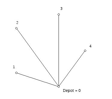Figure 6

We will assume that the trucks we are using have infinite capacity. Thus, we will be treating this problem as if what we are trying to do is find a TSP solution. We start by computing the savings that are associated with edges that connect two sites other than the depot (0).

S_1,2 = 31 + 33 - 40 = 24

S_1,3 = 31 + 37 - 61 = 7

S_1,4 = 31 + 29 - 46 = 14

S_2,3 = 33 + 37 - 42 = 28

S_2,4 = 33 + 29 - 49 = 13

S_3,4 = 37 + 29 - 48 = 18

In sorted order, from larger to smaller savings, the edges are: 2,3; 1,2; 3,4; 1,4; 2,4; and 1,3.

Since edge 2,3 has the largest saving, we can replace the pairs of tours 0,2,0 and 0,3,0 by the merged tour 0,2,3,0.

We now have a diagram (Figure 7) that looks like:

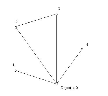Figure 7

The edge with the next largest saving is edge 1,2. This edge can be added to merge the tours 0, 1, 0 and 0, 2, 3, 0, to obtain the tour 0, 1, 2, 3, 0. We can see the resulting collection of tours at this stage in Figure 8.

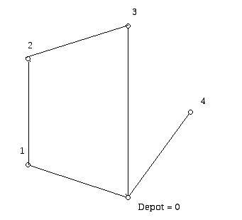Figure 8

The edge with the next largest sorted order would be 3,4. This edge can be used to merge the tours 0, 4, 0 and 0, 1, 2, 4, 0 to form a final tour, visiting all sites of 0, 1, 2, 3, 4, 0. Note that had 2, 4 been the cheapest edge at this stage it could not be used to merge the two tours. Had edge 1,4 been cheapest, then the merged tour would have been 0, 3, 2, 1, 4, 0 which visually is self-intersecting but permitted. Given the actual numbers here, the final tour is shown in Figure 9.

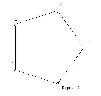Figure 9

The cost of this tour is 31 + 40 + 42 + 48 + 29 = 190.

A very commonly used heuristic for the TSP is known as nearest neighbor. Starting at the depot one goes next to that site not already visited for which the cost is the cheapest. In this example, nearest neighbor would select the sites in the order: 0, 4, 1, 2, 3, 0. This is a different tour from the one found using the Clarke-Wright heuristic. The cost of this tour is: 29 + 46 + 40 + 42 + 49 = 206 which is 16 units more expensive than the tour we found.

What would have to be done to find the optimal TSP tour for this example? You might want to see if you can find a cheaper tour than the one we found using the Clarke-Wright heuristic. To do so using brute force would involve examining all the possible TSP tours (there are (5)(4)(3)(2)(1)/2 = 60 possibilities; we divided by two since any tour is the same as the one read in reverse cyclic order).

Suppose there were goods to be collected at the sites:

1. 4 units
2. 2 units
3. 3 units
4. 1 unit

Also suppose that the vehicles have capacity 6.

What happens now when we apply Clarke-Wright? We can still use the same list edges sorted by savings. We again start with the tours 0, 1, 0; 0, 2, 0; 0, 3, 0; 0, 4, 0, which involve four vehicles but notice that each truck will pick up less than its capacity of 6. We can use edge 2,3 to merge the tours 0, 2, 0 and 0, 3, 0 because the pickups at 2 and 3 amount to 5 units, which is less than the capacity of the one truck that could serve these two cities. At this stage we have the tours 0, 1, 0; 0 (truck carries 4 units), 2, 3, 0 (truck carries 5 units) and 0, 4, 0 (truck carries 1 unit). Now the next largest saving is achieved with edge 1, 2. Although we can merge the tours 0, 1, 0 and 0, 2, 3, 0, neither of the trucks used for these smaller tours has the capacity for the combined load of 9, so we cannot merge these two tours. We move on to the edge with the next largest saving, edge 3, 4. Now this edge can be used to merge the tours 0, 2, 3, 0 and 0, 4, 0 and because the sum of the loads for these three sites (2, 3, and 1) is only 6, we can in fact combine these tours. At this stage we have the tours 0, 1, 0 (truck carries 4 units) and 0, 2, 3, 4, 0 (truck carries 6 units). No further merging of tours is possible so we terminate with two trucks and a total length of 31 + 31 (for tour 0, 1, 0) + 33 + 42 + 48 + 29 (for tour 0, 2, 3, 4, 0) = 214. It turns out this is not the optimal tour. Can you find a feasible tour which is cheaper?

You may also want to try using the other variant of Clarke-Wright on this problem to see if there is any difference in the tours found.

What is exciting about thinking about vehicle routing problems in conjunction with a specific example such as this one is that it suggests other methods for attacking this kind of problem as well as more general ideas for other types of combinatorial optimization questions. For example, in thinking about vehicle routing in general (or TSP problems with several salespersons) there are two different strategies that come to mind:

* cluster sites and then find good routes to visit the clusters

* find a cheap route (which may not meet other constraints) and then cluster to meet the necessary constraints.

Huge literatures exist for both of these strategies to solve VRP problems.

The reason why vehicle delivery questions are so complex is the large number of variables that come into play in providing the service that is needed. For example, here are some issues that must be taken into account in problems of this sort:

* Is the vehicle only making deliveries, or does the nature of the business also make sense for pickups to be allowed? Places where deliveries are to be made are known as linehaul sites and places where goods are to be picked up are known as backhaul sites. In some cases a problem may be purely a linehaul or backhaul but in other situations a mixture of customers is involved or there may be deliveries at some sites and pickups at the same site.

(Comments: When a truck is involved in making bread deliveries to restaurants, grocery stores, and supermarkets, it may appear that all that might be involved is that there would be different numbers of loaves that go to each of the "customers." However, there are restrictions on the dates that bread can be sold at a store. In such a case there may be dozens of breads which do not get sold or there may only be 2. The store may arrange to try to sell bread that is about to expire at a cheaper price the day before expiration, or it may be that if the number of breads is small it is cheaper to discard the breads than try to get them to a "soup kitchen." However, if the number of breads is big enough there may be a provision in the contract with the supermarket that these can be "returned." (The seller of the bread may have some legal way to use the outdated bread that can make the bread seller money.)

* Are there constraints on the times that deliveries or pickup can be made?

* There may be constraints of the total length of a tour (enough gasoline) or the number of sites on a particular tour.

* Special types of problems involve special kinds of trucks - firetrucks, dump trucks, milk tanker trucks, gasoline trucks, school buses, dial-a-ride buses, etc.

We have just scraped the surface of the multiple layers of issues that arise. New variants are being developed all the time; as computers become faster, problems which were beyond the reach of solution can now be solved. Mathematics is providing new methods and ideas for solving these new questions and making our lives richer and happier while at the same time keeping costs down and providing interesting new work within mathematics.

Keep on trucking!

References:

Applegate, D. and R. Bixby, V. Chvatal, W. Cook, The Traveling Salesman Problem: A Computation Study, Princeton U. Press, Princeton, 2007.

Buchsbaum, A. and G. Fowler, R. Giancarlo, Improving table compression with combinatorial optimization, Journal of the ACM 50 (2003) 825-851.

Ball, M. and T. Magnanti, C. Monma, G. Nemhauswer (eds.), Network Routing: Handbooks in Operations Research, Vol. 8, North-Holland, Amsterdam, 1995.

Balinski, M. and R. Quandt, On an integer program for a delivery problem, Operations Research, 12 (1964) 300-304.

Bodin, L. and B. Goldin, A. Assad, M. Ball, Routing and scheduling of vehicles and crews, the state of the art, Computers and Operations Research, 10 (1983) 63-212.

Christofides, N. and S. Eilon, An algorithm for the vehicle dispatching problem, Operational Research Quarterly, 20 (1969) 309-318.

Christofides, N. and A. Mingozzi, P. Toth, The vehicle routing problem, In N. Christofides, A. Mingozzi, P. Toth, C. Sandi, (eds.), Combinatorial Optimization, Wiley, Chichester, UK, 1979, pp 315-338.

Clarke, G. and J. Wright, Scheduling of vehicles from a central depot to a number of delivery points, Operations Research, 12 (1964) 568-581.

Crainic, T. and G. Laporte, Fleet Management and Logistics, Kluwer, Boston, 1998.

Dantzig, G. and J. Ramser, The truck dispatching problem, Management Science, 6 (1959) 80-91.

Dantzig, G. and J. Ramser, Optimum Routing of Gasoline Delivery Trucks, Proc. Fifth World Petroleum Cong., 1959, Section VIII, p. 19.

Fisher, M., Optimal solution of vehicle routing problems using minimum k-trees, Operations Research, 42 (1994) 626-642.

Fisher, M. and R. Jaikumar, A generalized assignment heuristic for the vehicle routing problem, Networks, 11 (1981) 109-124.

Garvin, W. and H. Crandall, J. John, R. Spellman, Applications of linear programming in the oil industry, Management Science, 3 (1957) 407-430.

Golden, B. and A. Assad, Vehicle Routing: Methods and Studies, North-Holland, Amsterdam, 1988.

Laporte, G. The vehicle routing problem: An overview of exact and approximate algorithms, European J. of Operational Research, 59 (1992) 345-358.

Laporte, G. and I. Osman, Routing Problems: A bibliography, Annals of Operations Research 61 (1995) 227-262.

Laporte, G. and Y. Norbet, Exact algorithms for the vehicle routing problem, Annals of Discrete Mathematics 31 (1987) 147-184.

Lawler, E. and J. Lenstra, A. Rinnooy Kan, D. Shmoys, (eds.), The Traveling Salesman Problem, Wiley, Chichester, UK, 1985.

Lenstra, J. and A. Rinnooy Kan, Some simple applications of the traveling salesman problem, Operational Research Quarterly, 26 (1975) 717-734.

Miller, D., A matching based exact algorithm for capacitated vehicle routing problems, ORSA J. of Computing 7 (1995) 1-9.

Toth, P. and D. Vigo, (eds.) The Vehicle Routing Problem, SIAM, Philadelphia, 2002.

Joseph Malkevitch
York College (CUNY)
malkevitch at york.cuny.edu

Those who can access JSTOR can find some of the papers mentioned above there. For those with access, the American Mathematical Society's MathSciNet can be used to get additional bibliographic information and reviews of some these materials. Some of the items above can be accessed via the ACM Portal , which also provides bibliographic services.