Voronoi Diagrams and a Day at the Beach

Posted August 2006.

Voronoi diagrams have been used by anthropologists to describe regions of influence of different cultures; by crystallographers to explain the structure of certain crystals and metals; by ecologists to study competition between plants; and by economists to model markets in the U.S. economy...

David Austin
Grand Valley State University
david at merganser.math.gvsu.edu

Mail to a friend

Print this article

Introduction

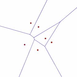
Suppose that you live in a desert where the only sources of water are a few springs scattered here and there. For each spring, you would like to determine the locations nearest that spring. The result could be a map, like the one shown here, in which the terrain is divided into regions of locations nearest the various springs.

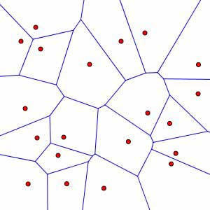
Maps like this appear frequently in various applications and under many names. To mathematicians, they are known as Voronoi diagrams. The locations of the springs are known, more generally, as sites and the set of points nearest a site is its Voronoi cell. Here is a program that shows how the diagram changes as the sites move.

Voronoi diagrams are rather natural constructions, and it seems that they, or something like them, have been in use for a long time. For instance, Descartes included the following figure with his demonstration of how matter is distributed throughout the solar system.

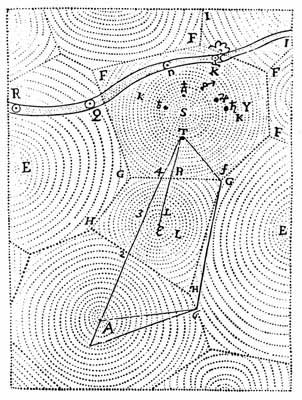
Since that time, Voronoi diagrams have been used by anthropologists to describe regions of influence of different cultures; by crystallographers to explain the structure of certain crystals and metals; by ecologists to study competition between plants; and by economists to model markets in the U.S. economy.

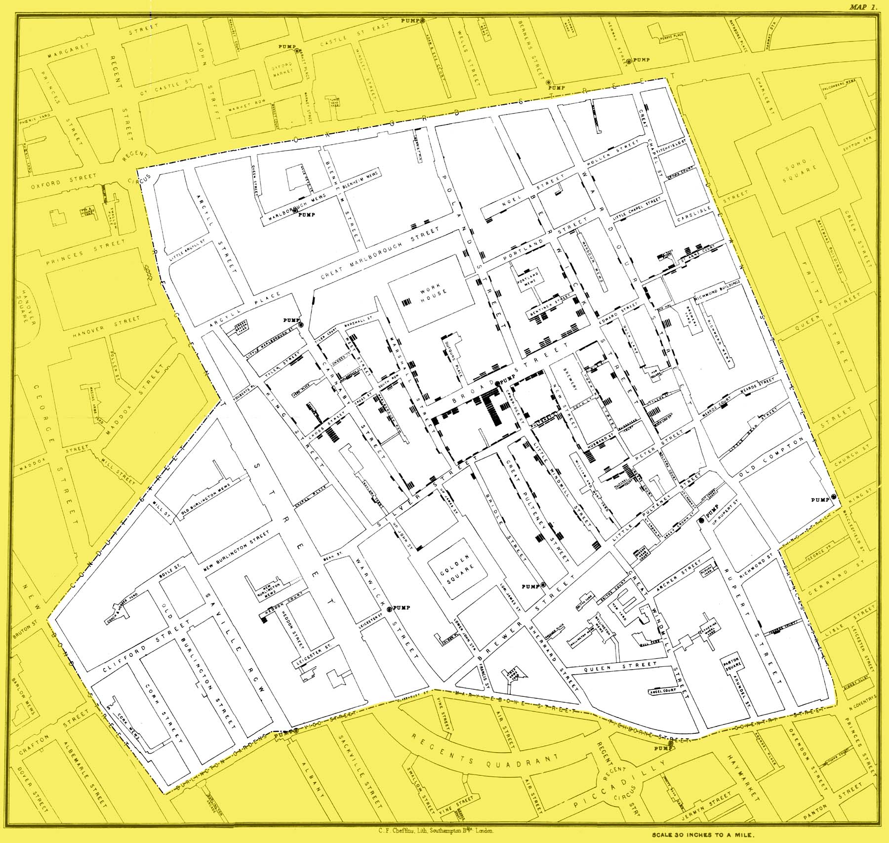
A particularly noteworthy application appears in John Snow's analysis of the London cholera outbreak of 1854. The following map, included in Snow's Report on the Cholera Outbreak in the Parish of St. James, Westminster, During the Autumn of 1854, shows the distribution of deaths due to cholera. Each bar represents a death at that address.

Click to enlarge

Snow then considered the sources of drinking water, pumps distributed throughout the city, and drew a line labeled "Boundary of equal distance between Broad Street Pump and other Pumps," which essentially indicated the Broad Street Pump's Voronoi cell.

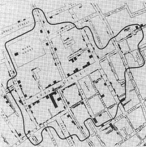
This map supported Snow's hypothesis that the cholera deaths were associated with contaminated water, in this case, from the Broad Street Pump. Snow recommended to the authorities that the pump handle be removed, after which action the cholera outbreak quickly ended. As Snow's work helped develop the modern field of epidemiology, this map has been called "the most famous 19th century disease map."

Constructing Voronoi diagrams

In this article, we'll imagine we are given a finite collection of sites and will see how to efficiently construct its Voronoi diagram.

When first confronted with this problem, it may seem most straightforward to consider every pair of points. An important fact is that if we are given two points $p$ and $q$ , then the perpendicular bisector of the line segment joining those two points consists precisely of the points that are the same distance from $p$ as from $q$ .

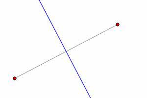
In fact, we may want to think of the perpendicular bisector as dividing the plane into two half-planes, one containing the points that are closer to $p$ and the other containing the points that are closer to $q$ .We will use ${\bf H}_p(q)$ to denote the half-plane containing the points that are closer to $p$ .

Constructing the Voronoi diagram then seems rather simple: to find the collection of points that are closer to $p_i$ than any other site, we simply take the intersection of all the half-planes ${\bf H}_{p_i}(p_j)$ . That is, the Voronoi cell containing the site $p_i$ is given by $\cap_j {\bf H}_{p_i}(p_j)$ .

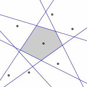
Of course, as the figure on the right shows, some of the work we are doing here is not necessary; that is, some of the sites that are relatively far away from $p_i$ have no influence on the Voronoi cell of $p_i$ . In fact, when there is a large number of sites, we would expect that the Voronoi cell of one particular point is determined by relatively few of the other sites.

If we use this method when there are $n$ sites, we need to consider the other $ n-1 $ sites to find the Voronoi cell of a particular site. Since each site has its own Voronoi cell, we need to construct $n$ Voronoi cells, which would require us to construct $n(n-1)=n^2-n\approx n^2$ half-planes. For instance, if we have 1000 points, we would need to construct approximately one million half-planes.

It appears that implementing this method will require us to do a lot of work, much of which is unnecessary. A natural question is whether there is a more efficient way to compute Voronoi diagrams.

Fortune's algorithm

In fact, there are several ways to find Voronoi diagrams, one of which is known as Fortune's algorithm.

This algorithm is based on the following clever idea: rather than considering distances between the various sites, we will introduce a line that moves through the plane and use this line to facilitate a more efficient comparison of distances. We call this line the sweep line and think of it as uncovering the Voronoi diagram as it sweeps through the plane.

Let's first remember that if we are given a point $p$ and a line $l$ (not containing $p$ ), then the set of points whose distance to $p$ equals its distance to $l$ forms a parabola.

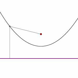
We will use $P_{p,l}$ to denote this parabola. As before, it is helpful to think of the parabola as dividing the plane into two regions: one consisting of points closer to $p$ and other consisting of points closer to $l$ .

This is an important point so let's make it a little more clear. Consider a point $q$ whose coordinates are $ q=(q_x,q_y) $ and whose distance to $p$ is denoted by $ d(q,p) $ . In what follows, the sweep line will always be a horizontal line; we will call its vertical coordinate $ l_y $ so that the distance between $q$ and $l$ is $ q_y-l_y $ . The condition that $q$ lies on the parabola $P_{p,l}$ is therefore

$d(q, p) = q_y-l_y$

or, more generally,

$ d(q, p) < q_y-l_y $ if $q$ lies above $P_{p,l}$ ,
$ d(q, p) = q_y-l_y $ if $q$ lies on $P_{p,l}$ , and
$ d(q, p) > q_y-l_y $ if $q$ lies below $P_{p,l}$ .

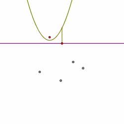
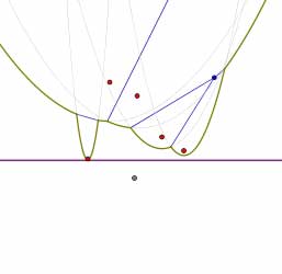
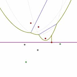
Now the horizontal sweep line $l$ will move down through the plane. At any time, we will only consider the sites that lie above the sweep line and the parabolas $P_{p,l}$ defined by those sites. For instance, given the collection of sites and the position of the sweep line shown on the left below, we will consider the parabolas as shown on the right.

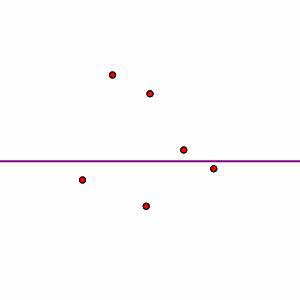
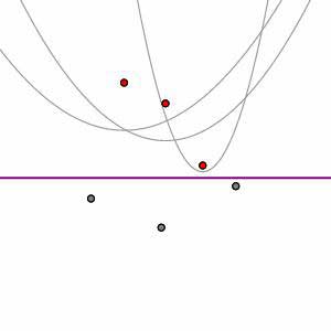
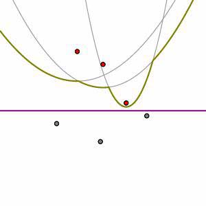
Now we can introduce the real star of Fortune's algorithm: the beach line is the curve formed by the lowest parabolic arcs. That is, any vertical line will pass through several parabolas; the point at which the vertical line passes through the beach line is the lowest such point. Notice that each of the arcs that composes the beach line is associated to one of the sites above the sweep line.

The beach line is well suited for constructing the Voronoi diagram. For instance, if a point lies above the beach line, it must be closer to one of the sites above $l$ than to $l$ . This means this point lies in the Voronoi cell of a site that the sweep line has already passed through. Therefore, the Voronoi diagram above the beach line is determined by the sites above the sweep line.

This may be a good time to look at an animation that shows how the beach line changes as the sweep line moves down through the plane.

Let's now determine when the beach line passes through some arbitrary point $q$ . Suppose that $q$ is as close to site $ p_1 $ as any other; that is, $d(q,p_1)\leq d(q,p_i)$ for all other sites $ p_i $ . The condition that $q$ lies on $P_{p_1,l}$ may be expressed as

$d(q,p_1) = q_y-l_y$

and therefore

$d(q, p_i)\geq d(q,p_1) = q_y-l_y$

This means that when $q$ appears on $P_{p_1,l}$ , it cannot be above another parabola $P_{p_i,l}$ . Therefore, when $q$ appears on the parabola $P_{p_1,l}$ , it is on the beach line. Let's summarize this important observation:

When a point appears on the beach line, it is on a parabolic arc associated to its nearest site.

The points on the beach line that lie on two parabolic arcs are called breakpoints. Applying our observation shows that the breakpoints are nearest two sites. In other words,

The breakpoints lie on the edges of the Voronoi diagram.

This means that the breakpoints will sweep out the edges of the Voronoi diagram as the sweep line moves down the plane. So to construct the Voronoi diagram, we simply need to keep track of the breakpoints. Here is an animation that shows how the edges are formed by the breakpoints.

Finding the edges

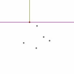
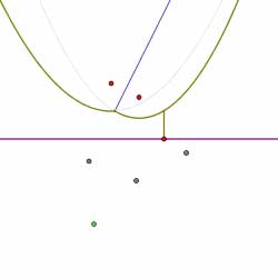
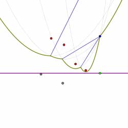
So far, we've seen that if we want to construct an edge of the Voronoi diagram, we simply need to keep track of the corresponding pair of breakpoints as the sweep line moves down the plane. The first step in doing this is to detect when a pair of breakpoints is constructed. This happens precisely when a new arc is added to the beach line as shown in the figures below.

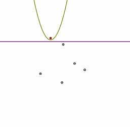
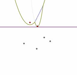
In other words, a pair of breakpoints corresponding to an edge in the Voronoi diagram appears on the beach line when the sweep line passes through a new site. We will call such an occurrence a site event.

Finding the vertices

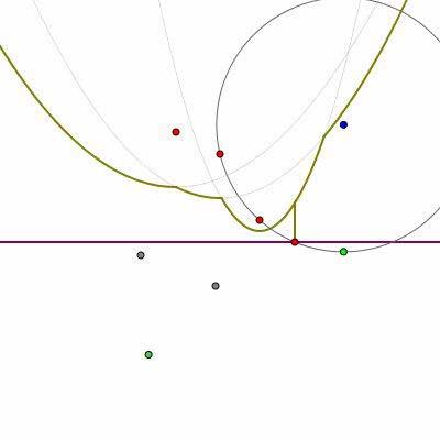
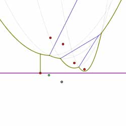
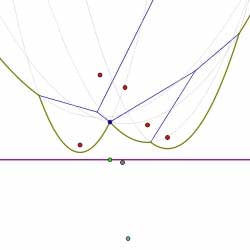
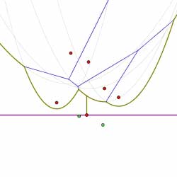
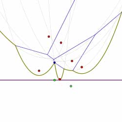
As the sweep line moves down, the breakpoints move continuously along an edge of the Voronoi diagram until they reach a vertex of the diagram. This happens when one of the parabolic arcs along the beach line disappears. In the following sequence of pictures, notice that the second parabolic arc from the right in the left figure (the smallest arc) disappears.

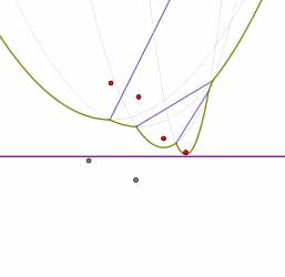
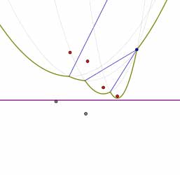
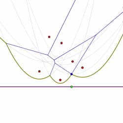
The appearance of new parabolic arcs on the beach line is easily detected: they occur when the sweep line passes through a site. Likewise, the disappearance of a parabolic arc is also easily detected. When a parabolic arc shrinks to a point $q$ , that point $q$ then lies on three parabolas: the one containing the disappearing arc and the two parabolas containing the arcs on either side. This means that $q$ is equidistant from three sites corresponding to these parabolas and that these three sites therefore lie on a circle centered at $q$ . We therefore find the vertex $q$ when the sweep line passes through the bottom of that circle.

We call such an occurrence a circle event. The change in the diagram therefore looks like this:

Notice that a new edge is also created by a circle event. This corresponds to the fact that we have a new breakpoint formed as the intersection of the two parabolic arcs that were adjacent to the disappearing arc.

The algorithm

We now have everything we need to know to understand Fortune's algorithm. To detect edges and vertices in the diagram, it is enough to find the appearance and disappearance of parabolic arcs in the beach line. We will therefore keep track of the beach line by imagining that we walk along it from left to right and record the order of the sites that produce its constituent parabolic arcs. We know that this order will not change until the sweep line reaches either a site event or circle event. Also, the breakpoints are implicitly recorded by noting the adjacency of the parabolic arcs on the beach line.

If the next event that the sweep line encounters is a site event, we simply insert the new site into our list of sites in the order in which the corresponding parabolic arc appears on the beach line. We then record the fact that we have encountered a new edge in the diagram.

If the next event that the sweep line encounters is a circle event, we record the fact that we have encountered a vertex in the diagram and that this vertex is the endpoint of the edges corresponding to the two breakpoints that have come together. We also record the new edge corresponding to the new breakpoint that results from the circle event.

Whether we encounter a site or circle event, we will always check to see if we have added a new triple of parabolic arcs on the beach line that may lead to a future circle event. It is also possible that we will remove a future circle event from consideration if the triple of parabolic arcs that led to it no longer exists after the event.

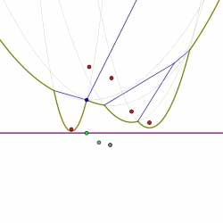
In this way, the diagram is constructed by considering the finite sequence of events. Shown below is the sequence of events that computes the Voronoi diagram of the collection of sites shown. Circle events are indicated by green dots.

Summary

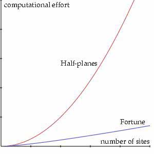
Fortune's algorithm is a remarkably efficient way to compute the Voronoi diagram. Whichever algorithm we use, we should expect that having more sites will require more work to find the Voronoi diagram. We can, however, be more precise about this. Earlier, we considered an algorithm for finding the Voronoi diagram by finding each Voronoi cell by intersecting each half-plane containing the site. If $ n $ is the number of sites, the number of steps required to implement this algorithm is proportional to $n^2\log n$ . For a typical diagram, however, the number of steps required to implement Fortune's algorithm is proportional to $n\log n$ , which represents a considerable improvement. The graph below compares the computational effort for these two algorithms depending on the number of sites.

References

M. de Berg, M. van Kreveld, M. Overmars, O. Schwarzkopf, Computational Geometry, Springer, 2000. Details for implementing Fortune's algorithm are given here.
Rene Descartes, Le Monde, ou Traité de la lumière, Translation and introduction by M.S. Mahoney, Abaris, 1979.
Ralph Frerich, ed., John Snow. A thorough and excellent web site, hosted by UCLA's Department of Epidemiology, devoted to John Snow. Permission to include the images of Snow's maps is gratefully acknowledged.
A. Okabe, B. Boots, K. Sugihara, S. Chiu, Spatial Tesselations, Concepts and Applications of Voronoi Diagrams, Wiley, 2000. A comprehensive treatment of Voronoi diagrams and related areas, including a survey of various applications and descriptions of several algorithms.
J. O'Rourke, Computational Geometry in C, Cambridge University Press, 2000.

David Austin
Grand Valley State University
david at merganser.math.gvsu.edu

NOTE: Those who can access JSTOR can find some of the papers mentioned above there. For those with access, the American Mathematical Society's MathSciNet can be used to get additional bibliographic information and reviews of some these materials. Some of the items above can be accessed via the ACM Portal, which also provides bibliographic services.