Finite Geometries?
Posted September 2006.
This will involve an excursion over a wide swath of the mathematical landscape and feature a variety of distinguished contributors to mathematics from many cultures...
Joe Malkevitch
York College (CUNY)
malkevitch at york.cuny.edu 
Introduction
The word "geometry," of Greek origin, means earth or land measure. As a branch of mathematics, geometry's standard definition concerns obtaining insights into shapes and the nature of space. Geometry has evolved into a rapidly growing field which is not merely concerned with shapes and space but more broadly with visual phenomena.
However, the shape of geometry as a mathematical subject was dramatically set by Euclid's Elements. This book develops geometry deductively, as a collection of logical conclusions deduced from a series of postulates or axioms, which are taken as self-evident truths. Scholars are unsure if Euclid thought of the Elements as "mathematical physics" or mathematics. Was Euclid saying that the theorems of the Elements about circles and triangles are the way the world is, or was he saying that in the mathematical world based on the assumptions he made, these are the conclusions that follow? To make the discussion more concrete, Euclid shows that a triangle must have angle sum 180 degrees. Did Euclid think that if one took three points in space, not on a line, and measured the angles in the triangle, he would get 180 degrees? Perhaps he realized that due to the impossibility of measuring anything with total accuracy, to show that the sum was exactly 180 would not be possible.
There is a lot of geometry being done which does not fit into the mold that Euclid set forth. Modern geometers think about symmetry questions, when various structures are rigid, how to move a robot from one place to another without hitting obstacles, and how to assign frequencies for cell phone conversations. But kinds of geometry much closer to what Euclid initiated are also being explored.
A model of a line segment, such as a stick of thin spaghetti, can be subdivided into smaller and smaller pieces, suggesting that there are infinitely many points that make up the line segment or spaghetti stick. However, in the view of contemporary physics, the spaghetti is made up of atoms and the subatomic particles that make up these atoms, so one is led to the idea that there are only a finite number, albeit very large, of atoms in the universe. Would it make sense to investigate a geometry where the axioms or rules talked about the existence of only a finite number of points and lines? Would it make sense to talk about finite geometries?
Mathematicians have indeed developed a sub-branch of mathematics concerned with finite geometries. This development was surprisingly recent in mathematics' history. I will here briefly look at how a theory of finite geometries developed. This will involve an excursion over a wide swath of the mathematical landscape and feature a variety of distinguished contributors to mathematics from many cultures.
Steiner Triple Systems
Mathematicians are trained to abstract and generalize. The physical origin of many mathematical problems tended to result in continuous models for problems arising outside of mathematics. Mathematical questions about counting, the collection of ideas that now belongs to the branch of mathematics called combinatorics, were developed surprisingly late in mathematics. Combinatorics became one part of the very rapidly growing part of mathematics known as discrete mathematics, which has especially blossomed under the influence of ideas from computer science. Many of these early combinatorial problems arose from attempts to solve problems that were raised as recreational mathematics questions.
As is often the case in mathematics, concepts and/or theorems are not named for the person who really deserves the credit. This happens partly because a term often comes into common usage in a time and place and takes root. If the earlier work is in another country or place it is not surprising that the credit is not quite accurate. Actually, the situation is complex. Someone may propose an idea and do nothing with it, while a later person popularizes the idea and makes a significant contribution.
The idea behind Steiner Triples is that one has a collection of objects S, which we will call points and will be represented here using positive integers. We want to create a set of three-element subsets of S, the set T (the triples) with the property that each pair of distinct elements in S appears in exactly one triple. In 1853 Jakob Steiner (1796-1863) raised the question of the existence of such set systems. That is, if |S| = v denotes the number of elements in set S, for what values of v does such a set of triples exist?
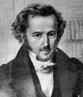
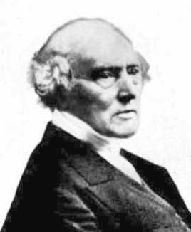
(Jakob Steiner)
Although this concept is attached to Jakob Steiner's name, in fact, the British mathematician Thomas P. Kirkman (1806-1895) had studied and already answered Steiner's question in 1847. Steiner is known for a variety of contributions to geometry, including work on isoperimetric problems (what region in the plane has the largest area with a fixed perimeter?) and projective geometry (geometry where all lines meet). Kirkman was one of the early pioneers of the study of combinatorics, the mathematics of counting problems, as well as an early investigator of the properties of 3-dimensional polyhedra from a point of view that took into account non-metrical considerations.
(The Reverend Thomas Penyngton Kirkman)
Here are two examples of such Steiner triple systems:
S1 = {1, 2, 3, 4, 5, 6, 7}
T1 = { {1, 2, 4}, {2, 3, 5}, {3, 4, 6}, {4, 5, 7}, {5, 6, 1}, {6, 7, 2}, {7, 1, 3} }
and
S2 = {1, 2, 3, 4, 5, 6, 7, 8, 9}
T2 = { {1,2, 3}, {4, 5, 6}, {7, 8, 9} | {1, 4, 7}, {2, 5, 8} {3, 6, 9} | {1, 5, 9}, { 2, 6, 7} {3, 4, 8} | {1, 6, 8}, {2, 4, 9}, {3, 5, 7}}
Note that for this second triple system, the three triples in the sets of triples between the vertical bars each lists the numbers one through nine exactly once. We will see later that these two triple systems were discovered in a natural way in an entirely different context.
Now let us return to the question of the existence of Steiner Triple Systems for various values of v, the size of the set S on which the triples are built. Notice that for the set {x, y, z} we can form three sets of two elements (e.g. {x, y}, {x, z}, {y, z}) and, furthermore, the set S contains v(v-1)/2 triples. Since every pair of distinct elements of set S appears in exactly one triple of set T, we have that 3|T| = v(v-1)/2. This means that |T| equals v(v-1)/6. Now, define T(x) to be the set of two-element sets obtained by locating the triples of T that contain x and removing x from those triples. For example, for the set of triples T1 above, T1(1) = { {2, 4}, {5, 6}, {3,7} }. In general, as illustrated by this example, T(x) partitions the elements of S with x removed into subsets with two elements. Hence, v - 1 must be an even number. Since v must therefore be odd, we have that v must leave a remainder of 1, 3, or 5 when divided by 6. The next step is to determine which numbers leave an odd remainder when divided by six for which one can construct a Steiner Triple System. The first such systemic construction was actually carried out by Kirkman. Others who have found nice methods for finding Steiner Triple Systems for some or all of the eligible values of v are R. C. Bose (1901-1987), Thoralf Skolem (1887-1963), and Richard Wilson. Skolem is best known for his work in logic.
(The Norwegian mathematician Thoralf Skolem)
The techniques involved in these constructions range from ideas involving graph theory to the use of Latin squares (square arrays in which the symbols in the array appear in each row and each column once), and to methods involving abstract algebra. Fans of Sudoku will be familiar with the concept of Latin squares.
Euclid in his Elements laid down the axioms (rules) that eventually became the basis for the modern treatment of "synthetic" Euclidean geometry. As amazing as Euclid's accomplishment was, a fully modern approach to Euclidean Geometry was not completed until the early part of the 20th Century when David Hilbert successfully completed a modern axiomatization of Euclidean geometry that built on the work of other geometers as Pappus, Desargues, Pasch, and others. What Hilbert accomplished was to give a collection of axioms that captures the "generally accepted" properties of Euclidean 3-dimensional geometry (with the geometry of the plane, thus, also included) but with the property that if any axiom A in his axiom set is replaced by its negation, ~A, one can give an interpretation of point and line for which the original rules with the axiom ~A holds! In what follows it will be convenient to concentrate on some of the essential incidence axioms of Euclidean geometry, those rules that capture the way points and lines behave, without some of the complicating rules for "betweenness" and "continuity." We do not need all the Hilbert Axioms to accomplish what we seek.
Here are stripped down versions of these rules:
(Affine 1). If P and Q are distinct points, there is a unique line m which contains P and Q.
(You can think of a line as a set which contains the points which make it up. A different approach is to use the concept of a "relation" and to define an "incidence relation" which provides the information about which points lie on which lines.)
(Affine 2). If P is a point not on a line m, there is a unique line l which passes through P and which contains no point of m.
(This means that l and m are parallel, that is, they have no point in common. The "parallel axiom" of Euclid's Elements is not phrased in this way. In the form started above the axiom has come to be known as Playfair's Axiom. It is only equivalent to Euclid's axiom in the presence of other additional axioms, and the relationship between different axioms and their statements is very subtle. For example, in the statement above the word "unique" appears but what is the consequence of omitting the word "unique?")
Although synthetic geometry (theorems deduced from axioms) was born in ancient Greece, analytical geometry was born much later through the work of Pierre de Fermat and René Descartes. Descartes showed that by representing a Euclidean point by a pair of real numbers (x, y) and a Euclidean line by an equation of the the form ax + by + c = 0 where not both of a and b are zero, one could also study properties of the Euclidean plane. Though some "facts" (e.g. theorems) are most clearly seen in synthetic form, other "facts" are mostly easily verified in analytical form. In particular, certain theorems can be varied in a relatively straightforward manner by "computation" in the analytical geometry situation. For example if one uses the coordinates (x1, y1), (x2, y2) and (x3, y3) as those of the vertices of a triangle, it is easy to verify that the coordinates of the point where the medians of the triangle meet are ((x1 + x2 + x3)/3, (y1 + y2 + y3)/3) while a synthetic proof of this requires more skill and in some ways yields more insight. On the other hand there is a transparent symmetry to the way that the analytical geometry gives its insight into this theorem.
Finite Arithmetics
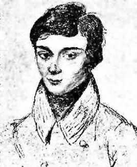
Given that numbers and number systems are at the very heart of mathematics, it is surprising that the development of finite arithmetics systems by the mathematics community came so late. It was Evariste Galois (1811-1832) who in conjunction with his efforts to show that polynomial equations of the fifth degree (quintics) could not be solved by providing formulas for their roots (as is true for polynomial equations of degree 1 to 4) first discovered the idea of finite arithmetics.
(Evariste Galois)
Finite arithmetics which obey all the algebraic rules (e.g. associativity, commutativity of addition and multiplication, etc.) of the real numbers are now known as finite fields, and are denoted GF( pn ) where p denotes a prime integer. The GF in this notation stands for Galois Field, which is another name given to these finite arithmetics. Amazingly, it has been shown that these are the only finite arithmetics which algebraically share the properties of the real or rational numbers. They are known to exist when the number of elements is a power of a prime, and for no other values. The breadth of applications of these finite fields is staggering, including such areas as error-correction and data compression systems that are essential for HDTV (high definition television) and cell phone technology.
One might have guessed that someone would have tried to mimic the definition of point and line used in analytical geometry but would restrict the numbers which were the coefficients of the variables to be elements from a finite field. This approach could have been used at this time to develop an analytical geometry of a finite affine plane. However, this step was not taken until much later. One tool to help develop the theory was the step of introducing homogeneous coordinates as a way to develop the analytical geometry of the real projective plane.
Steps towards finite geometry
Geometry made another big leap forward during the Renaissance when various artist-mathematicians laid down the foundations of projective geometry. One challenge these artists were trying to address was making more realistic looking images of buildings in their paintings. We are all familiar with the phenomenon that railroad tracks seem to meet in the distance when we know perfectly well they do not meet. The artists wanted to incorporate this perceptual reality into the way they represented scenes. Projective geometry, when axiomatized, a development that did not come immediately in the Renaissance, adopts two important axioms. The first of these axioms we have met before as axiom Affine 1:
(Projective 1). If P and Q are distinct points, there is a unique line m which contains P and Q.
The second axiom states:
(Projective 2). If l and m are distinct lines, then l and m have a point in common.
It is interesting to note that the synthetic development of projective geometry was carried out much earlier than the analytical version of projective geometry. In many areas of geometry visual insights into problems occur before methods to "algebratize" these visual insights are accomplished. Also, it is noteworthy that the two axioms for projective geometry are more symmetrical than those for affine geometry. Each of these axioms arises from the other by interchanging the role of point and line. This leads to the rich notion of duality in projective geometry. If one proves a theorem, then the statement obtained by interchanging the role of point and line will also be a theorem.
An important insight into Euclidean and projective geometry is the close relationship between the two. In an abstract framework where points and lines are treated as undefined terms and rules reflect the desired properties of these points and lines, then in a geometry where there are parallel classes of lines, that is, sets of lines where no pair of lines within a class meet, then one can proceed as follows. Let C be a class of parallel lines. For each such class we will add exactly one new point to our geometry. All of the new points that are added, one for each parallel class, are placed on a new single line. We now have a new geometry obtained from the old by adding some new points, modifying the old lines, and creating one new line. For those familiar with analytical geometry, it is well known that two lines are parallel if and only if they have the same slope or undefined slope (for vertical lines). Each real number, representing a slope, corresponds to one parallel class and there is one additional parallel class of the vertical lines. The line created with one point corresponding to each slope and one other point (for the vertical lines) is often referred to as the line "at infinity." If the original geometry is the Euclidean Plane, the new geometry obtained in this way is called the Real Projective Plane. It has infinitely many points and infinitely many lines. In particular the line at infinity has infinitely many points.
If one is given a projective plane, then one can reverse this construction by taking any line m and removing this line and modifying each of the lines of the plane by removing the one point on any line where that line meets m. (There must be such a point because in a projective plane every pair of lines meets.) The parallel classes in the new plane are obtained by noting that all the lines that meet at any point on m do not meet in the modified plane and are, thus, parallel. For the real projective plane the removal of any line gives rise to the Euclidean Plane, that is, all such planes are isomorphic (e.g. have the same structure). However, for general projective planes, the planes that are obtained by removing different lines need not be isomorphic.
The next major historical development occurred during the 19th century when Gauss, Bolyai and Lobachevsky developed what have come to be called the Bolyai-Lobachevsky Plane or hyperbolic geometry. This plane differs from the Euclidean plane in that through a point not on a line m there are many parallels to m. Eventually, researchers tried to construct finite analogues of the infinite hyperbolic plane. The theory of finite hyperbolic planes is much less far along than that of finite affine and projective planes.
Finite Geometries
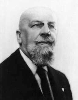
The earliest work on Finite Geometries has not been well charted by historians of mathematics. Part of this may be that one of the earliest contributors was Gino Fano (1871–1952), an Italian mathematician, who wrote almost exclusively in Italian. Fano constructed examples of finite projective planes and also finite spaces.
(Gino Fano)
Fano's work in the area of finite geometry included the discussion of a 3-dimensional finite geometry which consisted of 15 points, 35 lines, and 15 planes where each line had 3 points on it and each plane had 7 points. Fano had a long career as a teacher at the University of Turin, where he had also been a student. Due to his Jewish background he was forced out of his position in Turin and went to Switzerland for the war years. By the time the war was over Fano was quite elderly, but this did not prevent him from traveling to the United States and lecturing in Italy. Fano's sons Ugo and Robert had distinguished careers. Ugo earned a doctorate in mathematics but pursued a career in physics, and Robert taught engineering at MIT, where he did research on the mathematical problem of efficient data compression. The finite geometry shown in the diagram below is now called the Fano Plane in honor of Gino Fano.
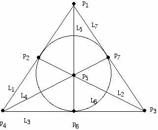
(Figure 1: One way of drawing a diagram representing the Fano Plane.)
A few comments are required to clarify the meaning of the diagram above. The Fano Plane has 7 points, and in the diagram above they are represented by the dark dots P1, ..., P7, which is a finite set of points. What are the lines of the Fano Plane? A typical line, say L7, consists of a set of three points. L7, as can be read from the diagram, consists of the points P1, P7, and P3. Looking at the way the diagram is drawn it may be tempting to think that the point P7 is "between" the points P1 and P3. However, this is not the case. Line L7 is a set of points but for this geometry we will not be able to give meaning to a concept of "betweenness." Also, the way that the line L7 has been drawn may make it appear as if there are lots of points between P7 and P1 but, in fact, this line has exactly three points on it. Many geometers like to have a diagram such as this figure to illustrate the Fano Plane but for those who find the diagram "confusing," one can revert to thinking of the Fano Plane as a set of 7 points and seven lines, where the exact points that make up each line have been specified.
Some people find another aspect of Figure 1 confusing. The line L6 also has three points on it: P7, P6, and P2. Yet this line is drawn as if it is a circle! Again, the diagram is an aid to insight and if one finds the fact that one of the lines is drawn in a "non-straight" fashion confusing, one can go back to just the set of points and the list of lines and points that make them up without using any diagram whatsoever. You may ask, why draw the line L6 as if it is circular? Is it possible to locate 7 points in the Euclidean plane in such a way that the points are in positions where all 7 lines of the Fano Plane lie along "straight" lines in the Euclidean plane? The answer is "no!" In fact, the diagram we have chosen is at least somewhat appealing because 6 of the 7 lines are represented as being on "straight" lines in the Euclidean plane.
If you are not happy with the diagram of the Fano Plane, you have already encountered this plane earlier in this article. It is the Steiner Triple System consisting of the sets S1 and T1 which we discussed earlier. In fact, the 7 sets making up T1 have labels which correspond exactly to the lines in Figure 1. I could have arranged for these two representations of the Fano Plane to be scrambled versions of each other. In that case, it would have been necessary to produce an isomorphism to show that the two "systems" were actually identical. It turns out that the Fano Plane is unique.
You should also verify that the points and lines displayed in Figure 1 obey the axioms Projective 1 and Projective 2 and, thus gives an example of a projective geometry. For example, if one takes the two points P6 and P2, the only line they lie on is L6. The lines L7 and L5 have only the point P1 in common. No lines in this geometry are parallel. All 7-point and 7-line finite projective geometries have the same structure. It turns out that for a finite projective plane with 17 points on each line, there are currently 13 known such planes, no pair of which are isomorphic. However, it is still unknown if this collection of 13 examples is all there are!
In our earlier discussion of projective planes we mentioned that it is possible to modify a projective plane to get a plane which has incidence properties that are like those of the Euclidean plane. Verify for yourself that if you omit, say, the line L7, then we get a geometry with 4 points and 6 lines. You may wish to write out the points and lines of the geometry so obtained and verify that the resulting geometry is isomorphic to the geometry in Figure 2 below.
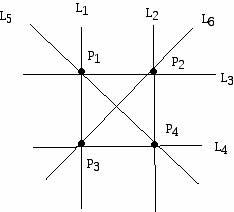
(Figure 2: A finite affine geometry with 4 points and 6 lines.)
The geometry in Figure 2 has four points and six lines and obeys the "Playfair" parallelism axiom. To help you understand the meaning of this diagram, note that if one chooses the point P1 which is not on line L6 (which consists of points P2 and P3), then the line L5 (consisting of points P1 and P4) contains P1 and is parallel to L6. It does not look as if L5 and L6 are parallel in Figure 2 but these lines are parallel in our finite affine geometry. The reason is that the point where these lines appear to meet is not a point of the geometry. Only the four points represented by dark dots are points of the geometry!
The Steiner triple system we looked at earlier, S2 and T2, turns out to be a finite affine plane with 3 points per line, 9 points, and 12 lines. You should convince yourself that this example satisfies the axioms Affine 1 and Affine 2. Using the terminology below, it is a plane of order 3.
The order of a finite affine plane is the number of points that lie on each line. It is not difficult to prove that in a finite affine plane if one line has n points on it, then all the lines must have exactly n points on them. Furthermore, the number of lines which go through each point must be exactly n + 1. Note that for a given point P not on line l there will be exactly one line through P which does not meet l, the line through P parallel to l. Based on the axioms it is not difficult to show that a finite affine plane of order n must have n2 points and n2 + n lines. For the very special affine plane that can be constructed as ordered pairs (x, y) from the n elements of a finite (Galois) field, it is apparent that there must be n2 points, since each coordinate can take on n values. In this plane it is also easy to see why there are n2 + n lines. Since a line is either vertical (there are n of these) or has the form y = mx + b, and there are n2 such lines (since m and b can each take on n different values), we have a total of n2 + n different lines. If a finite affine plane has n points on a line, it follows from the general construction for obtaining a projective plane from an affine plane (discussed earlier) that there are n + 1 points on every line of a finite projective plane. It is not difficult to see there are n2 + n + 1 points and n2 + n + 1 lines in any finite projective plane. Furthermore, there are n + 1 lines which pass through every point. Notice that one can count the number of points on a line and the total number of points and then get the number of lines through a point and the total number of lines by invoking the duality principle (once that principle has been proved).
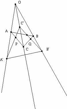
One of the most amazing theorems in the geometry of the real projective plane (the projective geometry derived from Euclidean geometry) was discovered by Girard Desargues (1591-1661). It states that if one has two triangles ABC and A'B'C' such that the points on the lines AA', BB' and CC' go through a single point O, then the lines AB and A'B', AC and A'C' and BC and B'C' meet in points R (not shown in Figure 3, but which would lie to the right of line OB'), P, and Q which lie on a single line! You should draw a diagram of this kind and verify that the three points P, Q, and R appear to be collinear, that is, lie on a single line. You should also formulate the dual theorem and converse theorem of Desargues' Theorem and convince yourself that these statements are valid in the real projective plane.
(Figure 3: Diagram illustrating Desargues' Theorem)
It turns out that while Desargues' "Statement" is true for a plane embedded in a 3-dimensional geometry and the real projective plane, there are infinite and finite projective planes where it does not hold. A simple example of such a plane is the Moulton Plane.
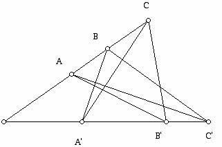
Closely associated with Desargues' Theorem is the wonderful theorem of the Alexandrian mathematician Pappus (born about 290, died about 350). Pappus' Theorem (projective plane version) states that given the three points A, B, and C on line l and A', B', and C' on line m, if segments AB' and A'B meet at R, BC' and B'C meet at P, and CA' and C'A meet at Q then P, Q, and R are collinear (e.g. lie on a line). The theorem is illustrated in Figure 4.
(Figure 4: Pappus' Theorem)
It turns out that Desargues' Theorem holds in a projective geometry if and only if that geometry can have coordinates introduced which obey the rules for a division ring. This is an algebraic structure which satisfies the usual algebraic properties of a field (for example, the real, rational or complex numbers are fields), except that commutativity of multiplication does not hold. It is also true that Pappus' Theorem holds in a projective geometry if and only if that geometry can be coordinatized using numbers from a field. Thus, it is possible to construct infinite projective planes where Pappus' Theorem holds but Desargues' does not. It turns out that every finite division ring is, in fact, a field. This lovely theorem is known as Wedderburn's Theorem. Thus, every finite Desarguean projective geometry is also Pappian. There is no known completely geometrical proof of this fact.
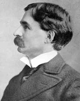
Putting together the various strands of affine and projective geometry and the way to deal with coordinates for dealing with finite spaces took a long time to develop. The mathematicians William Henry Bussey (who got his doctoral degree at the University of Chicago in 1904) and Oswald Veblen (who got his doctoral degree at the University of Chicago in 1903) were instrumental in the development of the subject.
(Oswald Veblen)
Veblen's doctoral thesis deals with axiomatic geometry. He has had nearly 5000 academic descendants. Veblen and Bussey were part of a movement in America, during the relatively early days of establishing a research mathematics community in the United States, which examined the foundations of geometry. Included was the mathematician E. H. Moore, who was Veblen's doctoral thesis advisor and who was an early president of the American Mathematical Society (AMS). Veblen also was president of the AMS. An important prize for research in geometry, administered by the AMS, is named for Veblen.
(Eliakim H. Moore)
We have discussed some of the properties of finite affine and finite projective planes. We have also shown that there is always such an affine plane for each value of n where n is a prime power because we can use coordinates from a finite field. Furthermore, when there is an affine plane with n points on a line there is also a projective plane with n + 1 points on a line. Certainly one major unsolved problem in the area of finite geometries is the question:
Are the only finite and projective planes of order n (n points and n +1 points on a line, respectively) those where n is a prime power?
Little progress has been made on this problem since it was first suspected to be true. There is a theorem due to Richard Bruck and Herbert Ryser which shows there are infinitely many integers which are not prime powers which can not be the order of a finite affine or projective plane. Using a computer search it was shown there can not be any projective plane of order 10 (e.g. 11 points on every line). The value 10 is the smallest number not ruled out by the Bruck-Ryser Theorem. However, no other facts are known.
In the approximately 100 years since the birth of work on finite geometries, the field has prospered and found multiple applications, many of which arise from the great symmetry of these planes. For example, the Fano Plane has 168 symmetries (more precisely, the group of its symmetries has order 168). In particular, the structure of finite geometries is often used in the branch of statistics devoted to the design of experiments. Finite geometries have been generalized in many ways. In particular, the theory of block designs has also found applications in a very wide variety of settings.
References
Albert, A., Finite planes for the high school, Mathematics Teacher 55 (1962) 165 - 169.
Anderson, I. Combinatorial Designs: Construction Methods, Ellis Horwood, 1993.
Batten, L., Combinatorics of Finite Geometries, Cambridge U. Press, 1986.
Beck, A., and M. Bleicher, D. Crowe, Excursions in Mathematics, Worth, New York, 1970. (Reprinted, A.K. Peters, 2000.)
Beth, T. and D. Jungnickel, and H. Lenz, Design Theory, Cambridge U. Press, London, 1986.
Botts, T., Finite planes and latin squares, Mathematics Teacher 54, (1961) 300 - 306.
Brown, E., The many names of (7, 3, 1), Mathematics Magazine, 75 (2002) 83-94.
Colbourn, C. and J. Dinitz, (eds.), The CRC Handbook of Combinatorial Designs, CRC Press, Boca Raton, 1996.
Dembowski, P., Finite Geometries, Springer-Verlag, New York, 1968.
Dénes, J. and A. Keedwell, Latin Squares and Their Applications, Academic Press, 1974.
Dinitz, J. and D. Stinson, (eds.), Contemporary Design Theory: A Collection of Surveys, John Wiley, New York, 1992.
Graves, L., A finite Bolyai-Lobachevsky planes, American Math. Monthly, 69 (1962) 130-132.
Heath, S., General finite geometries, Mathematics Teacher 64 (1971) 541 - 545.
Heath, S., The existence of finite Bolyai-Lobachevsky planes, Math. Mag., 43 (1970) 244-249.
Hughes, D. and F. Piper, Design Theory, Cambridge U. Press, London, 1985.
Jones, B., Miniature geometries, Mathematics Teacher, 52, (1959) 66 - 71.
Mac Neish, H., Four finite geometries, American Mathematical Monthly, 49 (1942), pp. 15-23.
Ostrom, T., Finite Translation Planes, Springer-Verlag, New York, 1970.
Polster, B, A Geometrical Picture Book, Springer-Verlag, New York, 1998.
Rosen, K. (ed.), Handbook of Combinatorial Mathematics, CRC, Boca Raton, 2000.
Ryser, H., Combinatorial Mathematics, Mathematical Association of America, Washington, 1963.
Wallis, W., Combinatorial Designs, Marcel Dekker, 1988.
Veblen, O. and W. Bussey, Finite Projective Geometries, Transactions of the AMS, 7 (1906) 241-259.
Additional references can be found here.
Joe Malkevitch
York College (CUNY)
malkevitch at york.cuny.edu
NOTE: Those who can access JSTOR can find some of the papers mentioned above there. For those with access, the American Mathematical Society's MathSciNet can be used to get additional bibliographic information and reviews of some these materials. Some of the items above can be accessed via the ACM Portal, which also provides bibliographic services.