Penrose Tilings Tied up in Ribbons
Posted December 2005.
How can we create a tiling by Penrose rhombs that will cover the entire plane...
David Austin
Grand Valley State University
david at merganser.math.gvsu.edu 
Introduction
While Penrose tilings are both mathematically interesting and aesthetically pleasing, constructing these tilings is a particularly important issue since they seem to model the structure of quasicrystals appearing in the natural world. As we saw in this space last August, however, constructing Penrose tilings is not easy for the first approach that comes to mind typically fails.
In this column, we will first review some of what was discussed in the previous column and then describe three methods for constructing Penrose tilings, each of which presents a different perspective on the tilings.
A quick review
For the purposes of this column, we will concentrate on the tilings by Penrose rhombs:
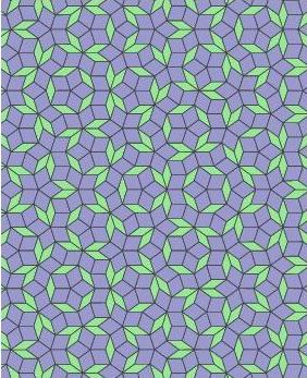
There are two types of tiles, typically called thick and thin rhombs. When placing tiles, we will require that certain matching rules be obeyed: we imagine that the edges of the tiles are decorated with arrows, as shown below, and we require that the arrows on adjacent edges agree in both number and direction.

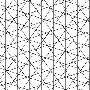
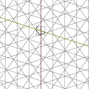
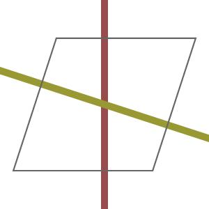
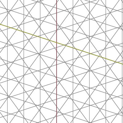
With this additional requirement, we saw that Penrose tilings admit no translational symmetry. This means that there is no fundamental unit that can reconstruct the tiling through repetition in the way that, say, the tiling below can be reconstructed from one of the yellow parallelograms.
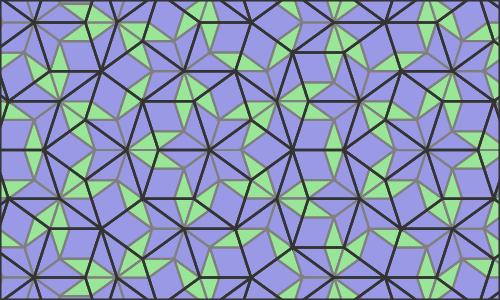
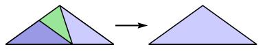
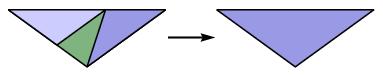
In spite of the fact that Penrose tilings have no translational symmetries, they do exhibit a remarkable structure. If we focus attention on half-rhombs, as shown below,

the matching rules force every half-rhomb to belong to one of the following patches:


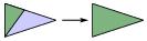
In this way, the half-rhombs may be combined, through a process known as composition, to obtain new half-rhombs whose linear dimensions are scaled by a factor of the golden ratio  , one of mathematics' revered numbers.
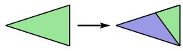
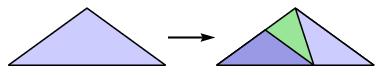
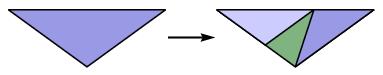
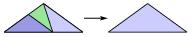
There is, of course, the reverse process of decomposition, in which a half-rhomb is replaced by smaller half-rhombs.
Through composition, a tiling by Penrose rhombs creates another tiling by larger Penrose rhombs, called the inflated tiling.
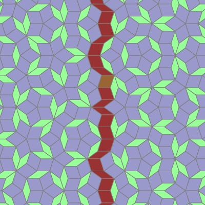
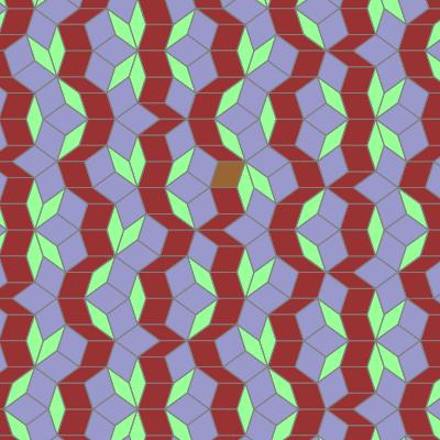
Composition applied to the inflated tiling creates its own inflated tiling, and, continuing in this way, we see that there is a hierarchy of tilings, each of which is the inflated tiling of its predecessor. This hierarchy imposes strong constraints on how we may place the tiles. More specifically, we saw that simply placing tiles according to the matching rules usually leads to a situation in which a patch of tiles cannot be extended further as happens in the following figure at the location indicated by the red dot.

The question remains: how can we create a tiling by Penrose rhombs that will cover the entire plane? We will now describe three different methods, each due to de Bruijn.
Updown generation
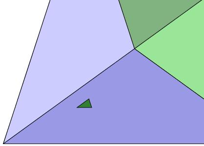
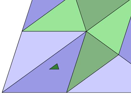
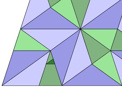
The first method, known as updown generation, is demonstrated with an example.
It should be apparent why this method is called updown generation: We first move up in the inflation hierarchy as we make choices about composing half-rhombs, then use decomposition to move back down the inflation hierarchy. Of course, we have made a finite sequence of choices here and consequently have covered only a finite portion of the plane. If we had continued so as to create an infinite sequence of composition choices, we would most likely have filled the entire plane. (There are some infinite sequences that cover only a portion of the plane, say, a half-plane, but these sequences are the exceptions.)
Besides providing a specific technique for constructing Penrose tilings, updown generation shows that there are many distinct Penrose tilings. While moving up the inflation hierarchy, there are several choices we can make at each step and hence there are infinitely many composition sequences. This implies that there is an infinitude--in fact, an uncountable infinitude--of distinct Penrose tilings.
The pentagrid method
You may feel a bit dissatisfied with updown generation: as we move up the inflation hierarchy, we cover larger and larger portions of the plane but, with only finitely many steps, never the entire plane. You may ask, "Is there a way to construct a tiling using just a finite amount of information?" De Bruijn's pentagrids provide such a method.
|
To understand how this method works, let's begin with an observation. First, opposite sides of a rhomb are parallel to one another. Therefore, if we begin with a rhomb and a pair of opposite sides, we may form a "ribbon" by adding the rhombs attached to that pair of opposite sides and then continuing outward.
|
 |
|
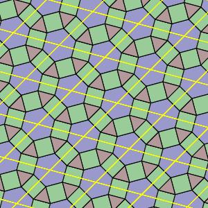
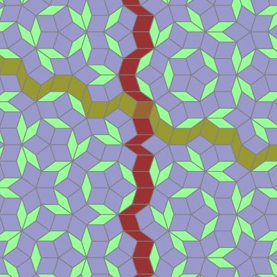
While there are, of course, many ribbons running through a tiling, they fall naturally into families of parallel ribbons consisting of ribbons that do not intersect. Since the sides of the rhombs may be aligned in five different directions, there are five such families of ribbons.
|
 |
|
Of course, every rhomb is defined by the intersection of two ribbons from different families.
|
 |
|
If you take a moment to study the ribbons, you may begin to feel they are a key that can unlock the structure of the tiling. In fact, de Bruijn noticed that the relationship between the ribbons can be used to describe the tiling. While the ribbons move through the tiling in a snaky sort of way, de Bruijn's fundamental insight is that it suffices, as we'll see, to represent the ribbons with straight lines. The intersection of two lines representing ribbons then defines a rhomb.
|
 |
|
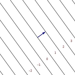
With this intuition in place, I will now describe the pentagrid method. First, if we are given a unit vector in the plane, we may consider a family of parallel lines perpendicular to the vector each of which is one unit away from its closest neighbors. Using the integers, we will label the regions between the lines in such a way that the label increases by one every time we cross a line in the direction of the unit vector. This family of parallel lines will model a family of ribbons in the tiling we are about to construct.
|
 |
|
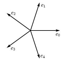
Now we will choose five unit vectors  where the angle between any two is a multiple of where the angle between any two is a multiple of  . .
|
 |
|
For each vector, we will consider the associated family of parallel lines where one line passes through the origin and the regions between the lines are labeled as described above. We will think of each family of parallel lines as a family of ribbons. However, some care is required for there are five lines intersecting at the origin and we know that, in a tiling, three or more ribbons cannot intersect. Therefore, we will choose real numbers  and translate the ith family of parallel lines by and translate the ith family of parallel lines by  so that no more than two lines intersect at a point. Indeed, most choices of real 5-tuples so that no more than two lines intersect at a point. Indeed, most choices of real 5-tuples  have this property. The resulting collection of lines, characterized by this 5-tuple, is called a pentagrid and leads to a Penrose tiling. have this property. The resulting collection of lines, characterized by this 5-tuple, is called a pentagrid and leads to a Penrose tiling.
|
 |
|
Since the lines in each family are to represent ribbons in the tiling, it should follow that the intersection of two lines corresponds to a rhomb. We will now see how this happens.
|
 |
|
Here is the intersection point from above drawn on a larger scale. For each family of lines, we have labeled the region between the lines with an integer. This means that the four regions around the intersection point are labeled by a 5-tuple of integers, one integer from each family of lines. To such a 5-tuple  we will associate the point in the plane we will associate the point in the plane  . .
|
 |
|
With this convention, we can see that the four points given by the four regions surrounding the intersection of the red and gold lines define a rhomb. Indeed, when we cross over the red line from left to right, we move in the direction  and when we cross over the gold line from bottom to top, we move in the direction and when we cross over the gold line from bottom to top, we move in the direction  . Therefore, the intersection point shown above defines the rhomb shown to the right. . Therefore, the intersection point shown above defines the rhomb shown to the right.
One sees that a thick rhomb is formed when the lines intersect at  and a thin rhomb is formed when the lines intersect at and a thin rhomb is formed when the lines intersect at  . Of course, this does not yet mean that a Penrose tiling is formed: We need to make sure that the matching rules are obeyed. Thankfully, de Bruijn checked this for us. The result is that a pentagrid, determined by the 5-tuple . Of course, this does not yet mean that a Penrose tiling is formed: We need to make sure that the matching rules are obeyed. Thankfully, de Bruijn checked this for us. The result is that a pentagrid, determined by the 5-tuple  , defines a Penrose tiling of the plane. , defines a Penrose tiling of the plane.
|
 |
For instance, the pentagrid on the left generates the tiling on the right.
Perhaps more remarkably, de Bruijn has proven that every Penrose tiling results from a pentagrid.
A curious fact
The pentagrid leads to a surprising fact about the relative number of thick and thin rhombs in a Penrose tiling. Your first thought may be that there are more thin rhombs; they are, after all, the smaller ones and so you might think that more of them are required to fill up little gaps that appear. However, we will see that the ratio of the number of thick rhombs to the number of thin rhombs is equal to the golden ratio  . In other words, it takes about 60% more thick rhombs than thin ones to construct a Penrose tiling. (Of course, there are infinitely many rhombs of both types; the precise meaning of the previous sentence will become clear presently.)
One consequence is that Penrose tilings are non-periodic, a fact that we determined through other means in August's column. In a periodic tiling with two tiles, the ratio of the number of one type to another must be a rational number equal to the ratio in a single fundamental unit.
Out of the shadows
There is an alternative point of view on the pentagrid method, usually called the projection method, that enables us to construct a Penrose tiling from a pentagrid as the "shadow" of a five-dimensional lattice. To see this, we will need to consider the five-dimensional space consisting of points with five real coordinates  . Don't worry if you can't see this five-dimensional space; we can draw some two-dimensional figures to help think about it.
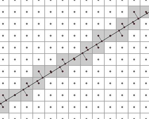
The point is that we may now forget about the original pentagrid and simply view the tiling as arising from the projection, or the "shadows," of the chosen lattice points onto the plane  .
.
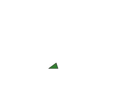
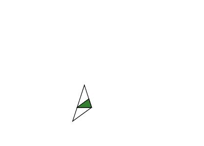
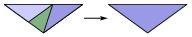
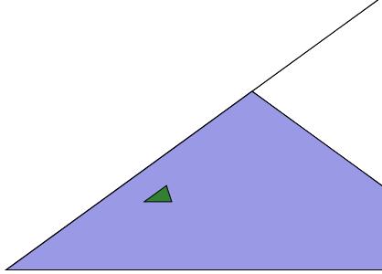
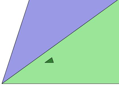
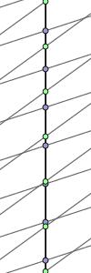
Incidentally, we have used a two-dimensional analogy to illustrate the projection method in the sequence of figures shown above. The slope of the line was chosen to be  , and the projection method results in a tiling of the real line, called a Fibonacci tiling, by a pair of one-dimensional tiles, sometimes called short (green) and long (blue) tiles. Fibonacci tilings are interesting in their own right for they are nonperiodic and appear naturally in Penrose tilings.
Summary
The methods of constructing tilings presented here have rather distinctive flavors. Updown generation shows how a small portion of a tiling may be grown to produce larger and larger portions. At any step of the process though, the entire tiling has not yet been determined. In contrast, the pentagrid method, and the related projection method, gives the complete structure of the tiling at a glance.
References
General references on Penrose tilings and inflation
- N.G. de Bruijn, Updown generation of Penrose tilings, Indagationes Mathematicae, New Series 1(2), 1990, 201-19.
- N.G. de Bruijn, Algebraic theory of Penrose's non-periodic tilings of the plane, Proceedings of the Koninklijke Nederlandse Akademie van Wetenschappen Series A, 84 (1), March, 1981, 39-66.
- M. Gardner, Extraordinary nonperiodic tiling that enriches the theory of tiles, Scientific American, January 1977, 110-121.
- B. Grünbaum and C.G. Shephard, Tilings and patterns, W.H. Freeman, New York, 1987.
- M. Senechal, Quasicrystals and geometry, Cambridge University Press, Cambridge, 1995.
- R. Penrose, Pentaplexity, Eureka 39, 1978, 16-22.
History and biography
- J.V. Field, Kepler's star polyhedra, Vistas Astronomy 23(2), 1979, 109-141.
- M. Senechal, The Mysterious Mr. Ammann, Mathematical Intelligencer 26, 2004, 10-21.
Quasicrystals
- R. Lifschitz, Introduction to quasicrystals
- D. Schechtman et al, Metallic phase with long range orientational order and no translational symmetry, Physical Review Letters 53, 1984, 1951-1954.
Nonlocal properties of Penrose tilings
- R. Penrose, Tilings and quasicrystals: a nonlocal growth problem?, in Introduction to the Mathematics of Quasicrystals, edited by Marko Jaric, Academic Press, 1989, 53-80.
- J. Socolar, Growth rules for quasicrystals, in Quasicrystals: the state of the art, edited by D. DiVincenzo and P.J. Steinhardt, World Scientific Publishers, 213-38.
David Austin
Grand Valley State University
david at merganser.math.gvsu.edu
NOTE: Those who can access JSTOR can find some of the papers mentioned above there. For those with access, the American Mathematical Society's MathSciNet can be used to get additional bibliographic information and reviews of some these materials. Some of the items above can be accessed via the ACM Portal, which also provides bibliographic services.


 . The distance
  between the intersection points is given by
  .
.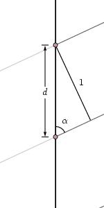
 in a line in our pentagrid, the number of intersections defining thick rhombs will be approximately
  while the number defining thin rhombs will be approximately
  . Therefore, the ratio of the number of thick rhombs to thin rhombs in this segment of length
  is approximately
![\[ \frac{h\sin72^\circ}{h\sin36^\circ} = \frac{\sin72^\circ}{\sin36^\circ} = \tau. \]](/featurecolumn/images/december05/index_22.gif)
 grows larger, this approximation becomes exact showing that the ratio of the number of thick rhombs to thin rhombs equals the golden ratio.
 , we will define a special two-dimensional plane
  that lies in five-space which is the plane containing the Penrose tiling we are constructing.
 , and there is a unique plane that this transformation rotates by
  . Translating this plane by the vector
  gives the plane
  .
. , it turns out the map that projects a point in five-space to its closest point in
  is given by
  . This projection map should remind you of how regions in the pentagrid define vertices in the Penrose tiling. We will therefore consider the lattice of points in five-space with integer coordinates for if we project some of these points into
  we will find the vertices of the tiling. A two-dimensional analogue of this situation is illustrated on the right; the plane
  is represented by the line.
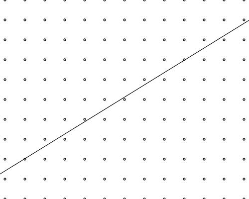

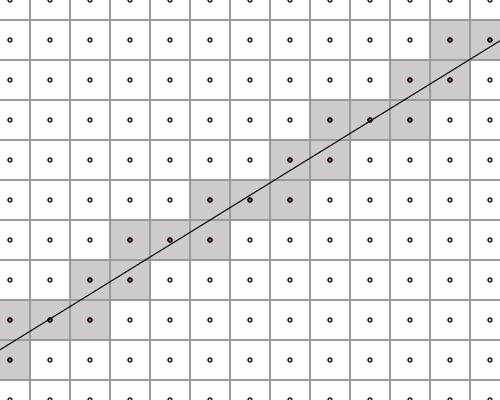
 are those whose Voronoi cell intersects the plane
  .
.
 .
.
 with the faces of the Voronoi cells.