A mixed multiscale finite element method for elliptic problems with oscillating coefficients

Abstract

The recently introduced multiscale finite element method for solving elliptic equations with oscillating coefficients is designed to capture the large-scale structure of the solutions without resolving all the fine-scale structures. Motivated by the numerical simulation of flow transport in highly heterogeneous porous media, we propose a mixed multiscale finite element method with an over-sampling technique for solving second order elliptic equations with rapidly oscillating coefficients. The multiscale finite element bases are constructed by locally solving Neumann boundary value problems. We provide a detailed convergence analysis of the method under the assumption that the oscillating coefficients are locally periodic. While such a simplifying assumption is not required by our method, it allows us to use homogenization theory to obtain the asymptotic structure of the solutions. Numerical experiments are carried out for flow transport in a porous medium with a random log-normal relative permeability to demonstrate the efficiency and accuracy of the proposed method.

1. Introduction

Many problems of fundamental and practical importance in science and engineering have multiple-scale solutions. Typical examples include composite materials with fine micro-structures and highly heterogeneous porous media. The direct numerical simulation of problems involving multiscale solutions is difficult, due to the requisite of tremendous amount of computer memory and CPU time, which can easily exceed the limit of today’s computer resources. On the other hand, in practice, it is often sufficient to predict the large scale solutions to a certain accuracy. Thus, various methods of upscaling or homogenization have been developed which replace the governing equations with multiscale solutions by the homogenized equations, whose solutions can be resolved on a coarse-scale mesh.

The recently developed multiscale finite element method 18, 19, 13 provides an effective way to capture the large-scale structures of the solutions on a coarse mesh. The central idea of the method is to incorporate the local small-scale information of the leading-order differential operator into the finite element bases. It is through these multiscale bases and the finite element formulation that the effect of small scales on the large scales is correctly captured. Apart from the computational advantages, such as saving in computer memory and good parallel efficiency 18 of the multiscale finite element method, we stress that the real significance of the method lies in its ability to solve the problems in coarse meshes. This is particularly advantageous when multiple simulations or realizations are necessary due to changes of boundary conditions or source functions for given fine microstructures of composite materials or highly heterogeneous permeability of porous media. Other relevant works on constructing special finite element bases can be found in 3 for layered microstructures and in 6 for convection-dominated diffusion problems.

The motivation of this paper is to explore the possibility of applying the multiscale finite element method to numerical computation of flow transport in highly heterogeneous porous media. In its simplest form, neglecting the effect of gravity, compressibility, capillary pressure, and considering constant porosity and unit mobility, the governing equations for the flow transport can be described by the following partial differential equations (see 21, 31, and 12):

$$\begin{eqnarray} & &\operatorname {div}({\mathcal{K}}(x)\nabla p)=0,{\tag{1.1}}\\ & &\frac{\partial S}{\partial t}+\mathbf{v}\cdot \nabla S=0, {\tag{1.2}} \end{eqnarray}$$

where $p$ is the pressure, $S$ is the water saturation, ${\mathcal{K}}(x)=({\mathcal{K}} _{ij}(x))$ is the relative permeability tensor, and $\mathbf{v}=-{\mathcal{K}} (x)\nabla p$ is the Darcy velocity. The highly heterogeneous properties of the medium are built into the permeability tensor ${\mathcal{K}}(x)$, which is generated through the use of sophisticated geological and geostatistical modeling tools. The detailed structure of the permeability coefficients makes the direct simulation of the above model infeasible. For example, it is common in real simulations to use millions of grid blocks, with each block having a dimension of tens of meters, whereas the permeability measured from cores is at a scale of centimeters 24. This gives more than $10^5$ degrees of freedom per spatial dimension in the computation. This makes a direct simulation to resolve all small scales prohibitive even with today’s most powerful supercomputers. On the other hand, from an engineering perspective, it is often sufficient to predict the macroscopic properties of the solutions. Thus it is highly desirable to derive effective coarse grid models to capture the correct large solution without resolving the small-scale features. Numerical upscaling is one of the commonly used approaches in practice. There are extensive studies in the literature on the numerical upscaling of two-phase flows through porous media, see, e.g., 1, 21, 11, 14, 30.

Mixed finite element approximations for second order elliptic problems, which approximate the source variable and flux simultaneously, have been studied by many authors (cf., e.g., 27 and the book 5). The local conservation of velocity flux is an important property in the mixed finite element methods. The violation of this local conservation property will lead to leakage of velocity flux. This will deteriorate the accuracy of the numerical solution for long-time computations. This is the reason why mixed finite element methods are attractive for porous medium simulations 28 (see also the numerical results in §5.1 of this paper). In this paper, we first propose and analyze a mixed multiscale finite element method with an over-sampling technique for solving elliptic equations with oscillating coefficients, and then apply the method to compute the above flow model 1.1-1.2. The use of the over-sampling technique is crucial in eliminating large resonance errors from the element boundaries. This point has already been well demonstrated in the previous study 1813 for the displacement multiscale finite element method. We will demonstrate that this technique applies also to the mixed multiscale finite element method. Our computational results show that the mixed multiscale method with the over-sampling technique gives more accurate results than the corresponding method without such technique.

We have performed careful numerical experiments to validate our mixed multiscale finite element method. To test how well our method works in a realistic application, we apply our method to a flow in porous media with a random log-normal relative permeability tensor. This is one of the practical benchmark test cases for oil recovery problems. Our computational results demonstrate convincingly the importance of the local conservation property in the flow simulation. When the local conservation property is not satisfied, the fractional flow curve deviates significantly from that obtained from the well-resolved mixed finite element calculation after a short time. The mixed multiscale finite element method, on the other hand, provides an accurate numerical approximation even on a coarse grid, with accuracy comparable to that obtained using the standard fine-mesh mixed finite element method. Finally, we compare the performance of the mixed multiscale method studied in this paper with the displacement multiscale finite element method studied in 18, 19, 13 when applied to the flow transport problem in heterogeneous porous media. The two methods give similar results at an early stage. But the fractional flow curve obtained by the displacement multiscale method deviates significantly from that obtained by the well-resolved calculation after a short time, clearly suffering from the violation of the local conservation property. The mixed multiscale method gives a more accurate solution than the displacement multiscale method for long-time calculations, due to the inherent local conservation property of the mixed multiscale method.

The ultimate goal of this study is to produce an effective coarse grid model for the two-phase flow with heterogeneous porous media. To this end, we need to upscale the saturation equation. Without capillary pressure, the saturation equation is hyperbolic. The effective equation is difficult to derive and has a nonlocal memory effect 29. Using an upscaling technique recently developed in 14 for the saturation equation, we show how the proposed mixed multiscale finite element method leads to a complete coarse grid algorithm. Our numerical results demonstrate convincingly that the fractional flow curve obtained from the resulting coarse grid model gives a very good approximation to that obtained from the fine grid calculation. Typically, many realizations on the same microstructure (permeability field) are made due to changes in boundary conditions and source fields. In such a case, the multiscale finite element bases are only constructed once, and can be used in the subsequent computations. Thus, the coarse grid model offers substantial saving in both memory and computing time. The saving could be as large as a factor of 10,000 if one can scale up by a factor of 10 in each space dimension (three space dimensions plus time).

The outline of the paper is as follows. In §2 we introduce the mixed multiscale finite element methods and present the main convergence results. In §3 we review the homogenization results for elliptic problems with Neumann boundary conditions. These results are the basis of our convergence analysis. In §4 we prove the error estimate for the mixed multiscale finite element method with over-sampling introduced in §2.3. The analysis depends on an abstract formulation for nonconforming mixed finite element methods, the homogenization theory, and a technique of “freezing coefficients” to deal with the local periodic coefficients. In §5 we apply our method to simulate the flow transport model 1.1-1.2 for a practical random log-normal permeability.

2. Mixed multiscale finite element methods

2.1. Notation and background

Let $\Omega$ be a polyhedral domain in $\mathbf{R}^d\ (d=2,3)$ with boundary $\partial \Omega$ whose unit outer normal is denoted by $\mathbf{n}$. Let $D\subseteq \Omega$ be a domain in $\mathbf{R}^d$ with the Lipschitz boundary $\Gamma$. For each integer $m\ge 0$ and $1\le p\le \infty$, we denote by $W^{m,p}(D)$ the standard Sobolev space of real functions having all their weak derivatives of order up to $m$ in the Lebesgue space $L^p(D)$. The norm and the seminorm of $W^{m,p}(D)$ will be denoted by $\|\cdot \|_{m,p,D}$ and $|\cdot |_{m,p,D}$, respectively. As usual, when $p=2$, $W^{m,2}(D)$ is denoted by $H^m(D)$ with the norm $\|\cdot \|_{m,D}$ and the seminorm $|\cdot |_{m,D}$. In the following, we let $V(D)$ denote the subspace of $H^1(D)$ whose functions have zero average over $D$.

We consider the following second order elliptic equations with locally periodic coefficients 4:

$$\begin{eqnarray} L_\varepsilon u_\varepsilon \,:\,=-\frac{\partial }{\partial x_i}\Big (a_{ij}\Big (x,\frac{x}{\varepsilon }\Big )\frac{\partial u_\varepsilon }{\partial x_j}\Big )=f\ \ &\text{ in }& \Omega ,{\tag{2.1}}\\ -a\Big (x,\frac{x}{\varepsilon }\Big )\nabla u_\varepsilon \cdot \mathbf{n}=g\ \ &\text{ on }&\partial \Omega . {\tag{2.2}} \end{eqnarray}$$

In this paper the usual Einstein summation convention for repeated indices is used. Here, $\varepsilon$ is assumed to be a small parameter, and $a(x,x/\varepsilon )=(a_{ij}(x,x/\varepsilon ))$ is a symmetric matrix which satisfies the uniform ellipticity condition:

$$\begin{eqnarray} \gamma \,|\xi |^2\le a_{ij}(x,y)\xi _i\xi _j\le \gamma ^{-1}\,|\xi |^2\ \ \ \ \ \ \forall \xi \in \mathbf{R}^d,x\in \bar{\Omega },y\in \mathbf{R}^d, {\tag{2.3}} \end{eqnarray}$$

for some positive constant $\gamma$. Furthermore, we assume that $a_{ij}\in C^1(\bar{\Omega };C^1_p(\mathbf{R}^d))$, where $C^1_p(\mathbf{R}^d)$ stands for the collection of all $C^1(\mathbf{R}^d)$ periodic functions with respect to the unit cube $Y$.

Let $u_0$ be the solution of the homogenized problem of 2.1-2.2:

$$\begin{eqnarray} L_0 u_0:=-\frac{\partial }{\partial x_i}\Big (a_{ij}^*(x)\frac{\partial u_0}{\partial x_j} \Big )=f\ \ &\text{ in }&\Omega ,{\tag{2.4}}\\ -a^*(x)\nabla u_0\cdot \mathbf{n}=g\ \ &\text{ on }&\partial \Omega , {\tag{2.5}} \end{eqnarray}$$

where $a^*(x)=(a_{ij}^*(x))$ with

$$\begin{eqnarray} a^*_{ij}(x)=\frac{1}{|Y|}\int _Y a_{ik}(x,y)\Big ( \delta _{kj}-\frac{\partial \chi ^j}{\partial y_k}(x,y)\Big )\, dy, {\tag{2.6}} \end{eqnarray}$$

and $\chi ^j(x,y)$ is the periodic solution of the cell problem

$$\begin{eqnarray} \ \ \ \ \ \frac{\partial }{\partial y_i}\Big (a_{ik}(x,y)\frac{\partial \chi ^j}{\partial y_k}(x,y)\Big )= \frac{\partial }{\partial y_i}a_{ij}(x,y)\ \ \ \text{ in }Y,\quad \int _Y\chi ^j(x,y)\,dy=0. {\tag{2.7}} \end{eqnarray}$$

Here $\delta _{kj}$ is the Kronecker delta, i.e., $\delta _{kj}=1$ for $k=j$ and $\delta _{kj}=0$ for $k\not =j$. Note that in 2.7 $x$ plays the role of a parameter. However, since $a_{ij}(x,y)$ is differentiable in $x$, we can easily show that $\chi ^j(x,y)$ is also differentiable in $x$. The convergence property of $u_\varepsilon$ to $u_0$ will be studied in detail in the next section.

Throughout the paper we impose the following assumptions on the data:

(H1) $f\in H^1(\Omega )$, $g=\mathbf{q}_0\cdot \mathbf{n}$ on $\partial \Omega$ for some $\mathbf{q}_0\in H^1(\Omega )^d$.

(H2) Compatibility: $\int _\Omega \,f\,dx=\int _{\partial \Omega }\,g\,ds$.

We remark that the assumption on the boundary value $g$ is not very restrictive. For example, in the case when $\Omega$ is a convex polygon in $\mathbf{R}^2$ with sides $\Gamma _j, 1\le j\le J$, and $g\in \Pi ^{J}_{j=1}H^{1/2}(\Gamma _j)$, such a flux $\mathbf{q}_0$ can be constructed through $\mathbf{q}_0=-\nabla u^*$ with $u^*\in H^1(\Omega )$ being the solution of the equation $-\Delta u^*+u^*=0$ in $\Omega$ with the Neumann boundary condition $\nabla u^*\cdot \mathbf{n}=g$ on $\partial \Omega$. The regularity results in 17 then ensure $\mathbf{q}_0\in H^1(\Omega )$. We also stress that the explicit formula of such a flux $\mathbf{q}_0$ is not required in the definition of our methods.

Denote by $L^2_0(\Omega )$ the subspace of $L^2(\Omega )$ whose functions have zero average over $\Omega$, and let $H_0(\operatorname {div};\Omega )$ be the subspace of $H(\operatorname {div};\Omega )$ given by

$$\begin{equation*} H_0(\operatorname {div};\Omega )=\{\,\mathbf{v}\in L^2(\Omega )^d\,:\,\operatorname {div}\,\mathbf{v}\in L^2(\Omega ),\ \mathbf{v}\cdot \mathbf{n}=0\ \ \text{on }\partial \Omega \,\}. \end{equation*}$$

The norm of $H(\operatorname {div};\Omega )$ will be denoted by $\|\cdot \|_{\operatorname {div},\Omega }$. Let $\mathbf{p}_\varepsilon =-a(x,x/\varepsilon )\nabla u_\varepsilon$ and $a^{-1}(x,y)$ the inverse matrix of $a(x,y)$; then $\nabla u_\varepsilon =-a^{-1}(x,x/\varepsilon )\mathbf{p}_\varepsilon$. The mixed formulation to 2.1-2.2 then reads as follows: find a pair $(\mathbf{p}_\varepsilon ,u_\varepsilon )\in H(\operatorname {div};\Omega )\times L^2_0(\Omega )$ such that $\mathbf{p}_\varepsilon \cdot \mathbf{n}=g$ on $\partial \Omega$ and

$$\begin{eqnarray} & &(\operatorname {div}\mathbf{p}_\varepsilon ,v)=(f,v)\ \ \ \ \forall v\in L^2(\Omega ),{\tag{2.8}}\\ & &(a^{-1}(x,x/\varepsilon )\mathbf{p}_\varepsilon ,\mathbf{q})-(u_\varepsilon ,\operatorname {div}\mathbf{q})=0\ \ \ \ \forall \mathbf{q}\in H_0(\operatorname {div};\Omega ). {\tag{2.9}} \end{eqnarray}$$

Here $(\cdot ,\cdot )$ stands for the inner product of $L^2(\Omega )$ or $L^2(\Omega ) ^d$. The existence of a unique solution of problem 2.8-2.9 and its equivalence to 2.1-2.2 follow directly from the abstract Babuska-Brezzi theory 5, 27.

Let us assume that $\mathcal{T}_h$ is a regular and quasi-uniform partition of $\Omega$ into simplices. For any $K\in \mathcal{T}_h$, let $h_K$ be its diameter, $|K|$ its Lebesgue measure, $\boldsymbol{\nu }^K$ the unit outer normal to $\partial K$, and $\{e^K_j\}_{j=1}^{d+1}$ the surfaces or edges of $\partial K$ with $|e^K_j|$ being the measure of $e^K_j$. The mixed multiscale finite element method that we are going to introduce is closely related to the Raviart-Thomas elements 27. For any $K\in \mathcal{T}_h$, we denote by $RT_0(K)$ the lowest order Raviart-Thomas approximation of $H(\operatorname {div},K)$:

$$\begin{equation*} RT_0(K)=P_0(K)^d+\mathbf{x}\,P_0(K),\ \ \ \ \mathbf{x}=(x_1,\cdots ,x_d)^{\mathrm{T}}\in \mathbf{R}^d, \end{equation*}$$

where $P_0(K)$ is the constant element space. Let $\{R^K_i\}^{d+1}_{i=1}$ be the basis of $RT_0(K)$ which satisfies

$$\begin{eqnarray*} R^K_i\cdot \boldsymbol{\nu }^K=\left\{ \begin{array}{ccl} \displaystyle \frac{1}{|e^K_i|}&\text{ on }&e^K_i,\\0&\text{ on }&e^K_j,j\not = i. \end{array}\right. \end{eqnarray*}$$

Since $\operatorname {div}R^K_i$ is constant in $K$, it follows easily from Green’s formula that $\operatorname {div}R^K_i=1/|K|$. Let $W_h\subset H(\operatorname {div};\Omega )$ be the lowest order Raviart-Thomas finite element space. It is well-known that there exists an interpolation operator $r_h:H(\operatorname {div},\Omega ) \cap H^1(\Omega )^d\to W_h$ such that $r_K:=r_h|_K$ satisfies the relations

$$\begin{eqnarray} \int _{e^K_j}\,(r_K\mathbf{q}-\mathbf{q})\cdot \boldsymbol{\nu }^K\,ds=0\qquad \forall \mathbf{q}\in H^1(K)^d,\ \ j=1,\cdots ,d+1, {\tag{2.10}} \end{eqnarray}$$

and the error estimate

$$\begin{eqnarray} \|\mathbf{q}-r_K\mathbf{q}\|_{m,K}\le Ch_K^{1-m}|\, \mathbf{q} \,|_{1,{K}}\quad \forall \mathbf{q}\in H^1(K)^d,\ \ m=0,1. {\tag{2.11}} \end{eqnarray}$$

Let $M_h\subset L^2_0(\Omega )$ be the standard piecewise constant finite element space for approximating $u_\varepsilon$. Then the standard mixed finite element method using the lowest order Raviart-Thomas element leads to the following discrete problem: find a pair $(\mathbf{p}_h,u_h)\in W_h\times M_h$ such that $\mathbf{p}_h\cdot \mathbf{n}=r_h\mathbf{q}_0\cdot \mathbf{n}$ on $\partial \Omega$ and

$$\begin{eqnarray*} & &(\operatorname {div}\mathbf{p}_h,v_h)=(f,v_h)\ \ \ \ \forall v_h\in M_h,\\ & &(a^{-1}(x,x/\varepsilon )\mathbf{p}_h,\mathbf{q}_h)-(u_h,\operatorname {div}\mathbf{q}_h)=0\ \ \ \ \forall \mathbf{q}_h\in W_h\cap H_0(\operatorname {div};\Omega ). \end{eqnarray*}$$

The following well-known error estimate can be obtained by using the Babuska-Brezzi theory 27, 5

$$\begin{eqnarray} \|\, \mathbf{p}_\varepsilon -\mathbf{p}_h \,\|_{\operatorname {div},{\Omega }}+\|\, u_\varepsilon -u_h \,\|_{0,{\Omega }}\le Ch(\|\, \mathbf{p}_\varepsilon \,\|_{1,{\Omega }} +\|\, u_\varepsilon \,\|_{1,{\Omega }}). {\tag{2.12}} \end{eqnarray}$$

Note that since $\|\, \mathbf{p}_\varepsilon \,\|_{1,{\Omega }}\le C\varepsilon ^{-1}$ 19, the error estimate 2.12 implies that the mesh size $h$ must satisfy $h<<\varepsilon$ to obtain accurate approximations. The purpose of the mixed multiscale finite element methods to be introduced next is to remove such a strong requirement on the mesh size $h$. This is achieved by building the local small-scale information into the finite element bases.

2.2. Mixed multiscale finite element method

Recalling that $V(K)$ denotes the subspace of $H^1(K)$ whose functions have zero average over $K$, we define $w^K_i\in V(K)$ as the solution of the following Neumann problem over $K$, for $i=1,\cdots ,d+1$:

$$\begin{equation} \int _K a\Big (x,\frac{x}{\varepsilon }\Big )\nabla w^K_i\nabla \varphi \,dx=\frac{1}{|K|}\int _K\varphi \,dx -\frac{1}{|e^K_i|}\int _{e^K_i}\varphi \,ds\quad \forall \varphi \in H^1(K), {\tag{2.13}} \end{equation}$$

Equation 2.13 is the weak formulation of the following boundary value problem

$$\begin{eqnarray*} L_\varepsilon \,w^K_i=\frac{1}{|K|}\ \ \text{in }K,\ \ -a\Big (x,\frac{x}{\varepsilon }\Big )\nabla w^K_i\cdot \boldsymbol{\nu }^K=\left\{ \begin{array}{cll} \displaystyle \frac{1}{|e^K_i|}&\text{ on }&e^K_i;\\0&\text{ on }&e^K_j,\ j\not = i. \end{array}\right. \end{eqnarray*}$$

Now let $\mathbf{p}^K_i=-a(x,x/\varepsilon )\nabla w^K_i$ and denote by $\operatorname {MS}(K)$ the multiscale finite element space spanned by $\mathbf{p}^K_i,i=1,\cdots ,d+1$. Recall that $\operatorname {div}R^K_i = \frac{1}{|K|}$. We have

$$\begin{equation*} \operatorname {div}\mathbf{p}^K_i=\operatorname {div}R^K_i\ \ \text{in }K,\quad \text{and}\quad \mathbf{p}^K_i\cdot \boldsymbol{\nu }^K= R^K_i\cdot \boldsymbol{\nu }^K\ \ \text{on }\partial K. \end{equation*}$$

Moreover, for any $\mathbf{q}_h\in \operatorname {MS}(K)$, the relations

$$\begin{equation*} \int _{e^K_i}\,\mathbf{q}_h\cdot \boldsymbol{\nu }^K\,ds=0,\ \ \ \ i=1,\cdots ,d+1, \end{equation*}$$

imply $\mathbf{q}_h=0$ in $K$. The degrees of freedom for $\mathbf{q}_h\in \operatorname {MS}(K)$ can be chosen as the zeroth order moments of $\mathbf{q}_h\cdot \boldsymbol{\nu }^K$ on the sides or faces of $K$. In practical applications, the base functions $\mathbf{p}^K_i$ of $\operatorname {MS}(K)$ will be approximated by solving 2.13 on a triangulation of $K$ with a mesh size resolving $\varepsilon$ using the lowest-order Raviart-Thomas mixed finite element method.

Let $\Sigma =H(\operatorname {div};\Omega )$, $Q=H_0(\operatorname {div};\Omega )$, and $M=L^2_0(\Omega )$. We define $\Sigma _h$ as the following multiscale finite element space for approximating the flux $\mathbf{p}_\varepsilon$:

$$\begin{equation*} \Sigma _h=\{\,\mathbf{q}_h\in H(\operatorname {div};\Omega ):\,\mathbf{q}_h|_K\in \operatorname {MS}(K),\forall K\in \mathcal{T}_h\,\}. \end{equation*}$$

Let $Q_h=\Sigma _h\cap Q$. To introduce an approximation of the boundary data $g$, we let ${\mathcal{B}}_h$ be the collection of all sides or faces of the triangulation $\mathcal{T}_h$ which lie on the boundary $\partial \Omega$. For any $e\in {\mathcal{B}}_h$ such that $e=\partial K\cap \partial \Omega$, we let $\mathbf{p}_e\in \operatorname {MS}(K)$ be the corresponding multiscale basis and define $g_h=\mathbf{q}_{0,h}\cdot \mathbf{n}$ on $\partial \Omega$ with $\mathbf{q}_{0,h}\in \Sigma _h$ given by

$$\begin{eqnarray*} \mathbf{q}_{0,h}=\sum _{e\in {\mathcal{B}}_h}\,\Big (\int _e\,g\,ds\Big )\,\mathbf{p}_e. \end{eqnarray*}$$

We can now introduce the following discretization of 2.8-2.9: find a pair $(\mathbf{p}_h,u_h)$ $\in \Sigma _h\times M_h$ such that $\mathbf{p}_h\cdot \mathbf{n}=g_h$ on $\partial \Omega$ and

$$\begin{eqnarray} & &(\operatorname {div}\mathbf{p}_h,v_h)=(f,v_h)\ \ \ \ \forall v_h\in M_h,{\tag{2.14}}\\ & &(a^{-1}(x,x/\varepsilon )\mathbf{p}_h,\mathbf{q}_h)-(u_h,\operatorname {div}\mathbf{q}_h)=0\ \ \ \ \forall \mathbf{q}_h\in Q_h. {\tag{2.15}} \end{eqnarray}$$

We have the following theorem concerning the convergence of this discrete problem.

Theorem 2.1.

The discrete problem 2.14-2.15 has a unique solution $(\mathbf{p}_h,u_h)\in \Sigma _h\times M_h$ such that $\mathbf{p}_h\cdot \mathbf{n}=g_h$ on $\partial \Omega$. Moreover, if the homogenized solution $u_0\in H^2(\Omega ) \cap W^{1,\infty }(\Omega )$ and the assumptions (H1)-(H2) are satisfied, then there exists a constant $C>0$, independent of $h$ and $\varepsilon$, such that

$$\begin{eqnarray} & &\|\, \mathbf{p}_\varepsilon -\mathbf{p}_h \,\|_{\operatorname {div},{\Omega }}+\|\, u_\varepsilon -u_h \,\|_{0,{\Omega }}\\ &\le &C(h+\varepsilon )(\|\, u_0 \,\|_{2,{\Omega }}+\|\, f \,\|_{1,{\Omega }}+\|\, \mathbf{q}_0 \,\|_{\operatorname {div},{\Omega }}) +C\sqrt {\frac{\varepsilon }{h}}\,\|\, u_0 \,\|_{1,\infty ,{\Omega }}. {\tag{2.16}} \end{eqnarray}$$

The proof of this theorem is simpler than that of Theorem 2.2 below for the over-sampling mixed multiscale finite element method, and will be omitted. We remark that the error estimate 2.16 is uniform as $\varepsilon \to 0$, which is in strong contrast to the error estimate 2.12, which blows up as $\varepsilon \to 0$. We also observe that the error estimate 2.16 deteriorates when $\varepsilon$ is of the same order as the mesh size $h$. This is due to the boundary layer effect of the multiscale bases, that is, the mismatch of the oscillating structure of $\mathbf{p}_\varepsilon$ and the linear behavior of the finite element solution $\mathbf{p}_h$ on the boundaries $\partial K$, $K\in \mathcal{T}_h$. This phenomenon is called resonant error in 18. The resonant error can be significantly reduced by an over-sampling technique introduced in 18. The over-sampling technique is based on the observation that the width of the boundary layer is of order $O(\varepsilon )$. Thus, if one first constructs some intermediate base functions on a larger sample domain (with size larger than $(h+ O(\epsilon ))$) and uses only the interior information from these intermediate base functions to construct the actual computational bases, then the boundary layer effect can be substantially reduced, resulting in more accurate approximations.

2.3. Over-sampling technique

In this subsection we will use the over-sampling technique 18 to construct new multiscale finite element bases for which the boundary layer effect of the bases $\mathbf{p}^K_i,i=1,\cdots ,d+1$, is reduced.

For any $K\in \mathcal{T}_h$, we denote by $S=S(K)$ a macro-element which contains $K$ and satisfies following condition:

(H3)

$h_S\le C_0h_K$ and $\operatorname {dist}(\partial K,\partial S)\ge \delta _0 h_K$ for some positive constants $C_0,\delta _0$ independent of $h$. The minimum angle of $S(K)$ is bounded below by some positive constant $\theta _0$ independent of $h$.

Let $\{R^S_i\}^{d+1}_{i=1}$ be the basis of $RT_0(S)$ which satisfies

$$\begin{eqnarray*} R^S_i\cdot \boldsymbol{\nu }^S=\left\{ \begin{array}{ccl} \displaystyle \frac{1}{|e^S_i|}&\text{ on }&e^S_i,\\0&\text{ on }&e^S_j,j\not = i. \end{array}\right. \end{eqnarray*}$$

Recall that $V(S)$ stands for the subspace of $H^1(S)$ whose functions have zero average over $S$. Let $\{\mathbf{p}^S_i\}^{d+1}_{i=1}$ be the multiscale finite element basis of $\operatorname {MS}(S)$ defined as in 2.13, i.e., $\mathbf{p}^S_i=-a(x,x/\varepsilon )\nabla w^S_i$, where $w^S_i \in V(S)$ is the solution of the following problem over $S$, $i=1,\cdots ,d+1$:

$$\begin{equation} \int _S\,a\Big (x,\frac{x}{\varepsilon }\Big )\nabla w^S_i\nabla \varphi \,dx=\frac{1}{|S|}\int _S\,\varphi \,dx- \frac{1}{|e^S_i|}\int _{e^S_i}\,\varphi \,ds\ \ \ \ \forall \varphi \in H^1(S). {\tag{2.17}} \end{equation}$$

Then we define the over-sampling finite element basis over $K$ by

$$\begin{eqnarray} \bar{\mathbf{p}}^K_i=c^K_{ij}\mathbf{p}^S_j|_K\ \ \ \ \text{ in }K, {\tag{2.18}} \end{eqnarray}$$

where the constants $c_{ij}^K$ are chosen such that

$$\begin{eqnarray} R^K_i=c^K_{ij}R^S_j|_K. {\tag{2.19}} \end{eqnarray}$$

The existence of the constants $c_{ij}^K$ is guaranteed because $\{R^S_j\}_{j=1}^{d+1}$ also forms the basis of $RT_0(K)$. Since $\operatorname {div}\mathbf{p}^S_j=\operatorname {div}R^S_j=1/|S|$, we know that

$$\begin{eqnarray} \operatorname {div}\bar{\mathbf{p}}^K_i=\operatorname {div}R^K_i\ \ \text{in }K. {\tag{2.20}} \end{eqnarray}$$

Here again, in practical applications, the base functions $\mathbf{p}^S_i$ of $\operatorname {MS}(S)$ will be further approximated by solving 2.17 on a triangulation of $S$ with a mesh size resolving $\varepsilon$ using the lowest order Raviart-Thomas finite element method. When applying the multiscale finite element method to solve 1.1-1.2, these base functions can be precomputed initially to generate the coarse grid operator. So this will be only a small overhead of the overall computations. This is also a common practice in many upscaling methods 10, 11.

We define $X=\prod _{K\in \mathcal{T}_h}H(\operatorname {div};K)$ with norm $\|\mathbf{q}\|_X=(\sum _{K\in \mathcal{T}_h}\|\, \mathbf{q} \,\|_{\operatorname {div},{K}}^2)^{1/2}$. Let $\Lambda (K)=\operatorname {span}\{\bar{\mathbf{p}}^K_i\}^{d+1}_{i=1}$ and $\Pi _K:\Lambda (K)\to RT_0(K)$ be the projection

$$\begin{eqnarray*} \Pi _K\mathbf{q}=c_iR^K_i\ \ \text{ if }\ \ \mathbf{q}=c_i\bar{\mathbf{p}}^K_i\in \Lambda (K). \end{eqnarray*}$$

Let $\bar{X}_h$ be the finite element space

$$\begin{equation*} \bar{X}_h=\{\mathbf{q}_h\in X:\,\mathbf{q}_h|_K\in \Lambda (K),\ \ \forall K\in \mathcal{T}_h\} \end{equation*}$$

and define $\Pi _h:\bar{X}_h\to \prod _{K\in \mathcal{T}_h}RT_0(K)$ through the relation $\Pi _h\mathbf{q}_h|_K=\Pi _K\mathbf{q}_h$ for any $K\in \mathcal{T}_h$, $\mathbf{q}_h\in \bar{X}_h$. The over-sampling mixed multiscale finite element space for approximating the flux $\mathbf{p}_\varepsilon =- a(x,x/\varepsilon )\nabla u_\varepsilon$ is then defined as

$$\begin{equation*} X_h=\{\mathbf{q}_h\in \bar{X}_h:\Pi _h\mathbf{q}_h\in W_h\subset H(\operatorname {div};\Omega )\}. \end{equation*}$$

We remark that, in general, $X_h\not \subset \Sigma =H(\operatorname {div};\Omega )$. Here, we require $\Pi _h\mathbf{q}_h \in W_h$ to impose some intrinsic continuity of the zeroth order moment of the normal components of $\mathbf{q}_h\in X_h$ across the interelement boundaries of the triangulation $\mathcal{T}_h$. Finally, let $G_h$ be the closed subspace of $X_h$ defined by

$$\begin{equation*} G_h=\{\mathbf{q}_h\in \bar{X}_h:\Pi _h\mathbf{q}_h\in W_h\cap H_0(\operatorname {div};\Omega )\}. \end{equation*}$$

The over-sampling mixed finite element approximation of 2.14-2.15 can be formulated as follows: find a pair $(\mathbf{p}_h,u_h)\in X_h\times M_h$ such that $\mathbf{p}_h\cdot \mathbf{n}=\bar{g}_h$ on $\partial \Omega$ and

$$\begin{eqnarray} \ \ \sum _{K\in \mathcal{T}_h}\int _K\,a^{-1}\mathbf{p}_h\cdot \mathbf{q}_h\,dx -\sum _{K\in \mathcal{T}_h}\int _K\,\operatorname {div}\mathbf{q}_h\cdot u_h\,dx&=&0\ \ \ \ \forall \mathbf{q}_h\in G_h, {\tag{2.21}}\\ \sum _{K\in \mathcal{T}_h}\int _K\,\operatorname {div} \mathbf{p}_h\cdot v_h\,dx&=&(f,v_h)\ \ \ \forall v_h\in M_h. {\tag{2.22}} \end{eqnarray}$$

Here $\bar{g}_h=\bar{\mathbf{q}}_{0,h}\cdot \mathbf{n}$ is the approximation of the boundary value with $\bar{\mathbf{q}}_{0,h}\in X_h$ given by

$$\begin{eqnarray*} \bar{\mathbf{q}}_{0,h}=\sum _{e\in {\mathcal{B}}_h}\,\Big (\int _e\,g\,ds\Big )\, \bar{\mathbf{p}}_e, \end{eqnarray*}$$

for any $e\in {\mathcal{B}}_h$ such that $e=\partial K\cap \partial \Omega$, and $\bar{\mathbf{p}}_e\in \Lambda (K)$ is the corresponding over-sampling multiscale basis.

We have the following theorem about the convergence of the over-sampling mixed multiscale finite element method. The assumption (H4) will be made precise in §4, see equation 4.8. This is an assumption on the maximum bound of a boundary corrector term (in the multiple scale expansion) in terms of the gradient of the homogenized solution. The validity of this assumption can be easily proved for the corresponding Dirichlet boundary value problem, due to the maximum principle.

Theorem 2.2.

The discrete problem 2.21-2.22 has a unique solution $(\mathbf{p}_h,u_h)\in X_h\times M_h$ such that $\mathbf{p}_h\cdot \mathbf{n}=\bar{g}_h$ on $\partial \Omega$. Moreover, if the homogenized solution $u_0\in H^2(\Omega )\cap W^{1,\infty }(\Omega )$ and the assumptions (H1)-(H4) are satisfied, then there exist constants $\delta >0$ and $C>0$, independent of $h$ and $\varepsilon$, such that if $h_K\le \delta ,\varepsilon /h_K \le \delta$ for all $K\in \mathcal{T}_h$, the following error estimate holds:

$$\begin{equation*} \begin{split} & \|\, \mathbf{p}_\varepsilon -\mathbf{p}_h \,\|_{X}+\|\, u_\varepsilon -u_h \,\|_{0,{\Omega }}\\ &\qquad \le C(\varepsilon +h)(\|\, u_0 \,\|_{2,{\Omega }}+\|\, f \,\|_{1,{\Omega }}+\|\, \mathbf{q}_0 \,\|_{\operatorname {div},{\Omega }})\\ &\qquad \quad +C\Big (\frac{\varepsilon }{h}+\sqrt \varepsilon \Big )(\|\, u_0 \,\|_{1,\infty ,{\Omega }}+\|\, f \,\|_{0,{\Omega }}+\|\, \mathbf{q}_0 \,\|_{\operatorname {div},{\Omega }}). \end{split} \end{equation*}$$

The proof of this theorem, which will be given in §4, depends on an abstract formulation for nonconforming mixed finite element methods, the homogenization results for elliptic equations with locally periodic coefficients in §3, and a technique of “freezing coefficients” to deal with the local periodicity of the coefficients. This new technique can also be used to extend the convergence analysis in 19, 13 for displacement multiscale finite element methods to elliptic equations with locally periodic coefficients. We remark that locally periodic coefficients model a wide class of microstructures which include, in particular, the layered structures. Previous numerical experiments in 13 and our numerical experiments indicate that the over-sampling technique leads to significant improvement over the direct mixed multiscale finite element method 2.14-2.15.

3. Homogenization results

In this section we summarize some homogenization results for the Neumann problem in the form to be used in this paper.

Let $D\subseteq \Omega$ be a domain in $\mathbf{R}^d$ with Lipschitz boundary $\Gamma$. Given $f\in L^2(D)$ and $g\in L^2(\Gamma )$ which satisfy the compatibility condition

$$\begin{eqnarray} \int _D f\, dx = \int _\Gamma g\, ds, {\tag{3.1}} \end{eqnarray}$$

we consider the following Neumann problem with rapidly oscillating coefficients: find $w_\varepsilon \in V(D)$ such that

$$\begin{eqnarray} \int _D a\Big (x,\frac{x}{\varepsilon }\Big )\nabla w_\varepsilon \nabla \varphi \, dx = \int _D f\varphi \, dx-\int _\Gamma g\varphi \, ds\quad \forall \varphi \in H^1(D). {\tag{3.2}} \end{eqnarray}$$

It is well-known that this problem admits a unique solution in $V(D)$ due to the compatibility condition 3.1. Let $w_0\in V(D)$ be the unique solution of the homogenized problem

$$\begin{eqnarray} \int _D a^*(x)\nabla w_0\nabla \varphi \, dx = \int _D f\varphi \, dx-\int _\Gamma g\varphi \, ds\quad \forall \varphi \in H^1(D), {\tag{3.3}} \end{eqnarray}$$

where $a^*(x)$ is given by 2.6.

In the following we will assume that $w_0\in H^2(D) \cap W^{1,\infty }(D)$. This regularity is valid, for example, when $f\in L^p(\Omega )$, $g=\mathbf{q}_0\cdot \mathbf{n}$ on $\Gamma$ for some $\mathbf{q}_0\in W^{1,p}(\Omega )$, where $p>2$, and $D$ is a smooth domain 15 or a convex polyhedral domain in $\mathbf{R}^2$ or $\mathbf{R}^3$ 17, 23.

Now we set

$$\begin{equation*} w^\varepsilon _1(x)=w_0(x)-\varepsilon \chi ^k\Big (x,\frac{x}{\varepsilon }\Big )\frac{\partial w_0}{\partial x_k}, \end{equation*}$$

where $\chi ^k(x,y)$ is the solution of the cell problem 2.7. Then by simple calculations we get

$$\begin{eqnarray} a_{ij}\Big (x,\frac{x}{\varepsilon }\Big )\frac{\partial w^\varepsilon _1}{\partial x_j}&=&a_{ij}^*(x)\frac{\partial w_0}{\partial x_j} -G^k_i\Big (x,\frac{x}{\varepsilon }\Big )\frac{\partial w_0}{\partial x_k}{\tag{3.4}}\\ &-&\varepsilon a_{ij}\Big (x,\frac{x}{\varepsilon }\Big )\frac{\partial \chi ^k}{\partial x_j} \Big (x,\frac{x}{\varepsilon }\Big )\frac{\partial w_0}{\partial x_k}\\ &-&\varepsilon a_{ij}\Big (x,\frac{x}{\varepsilon }\Big )\chi ^k\Big (x,\frac{x}{\varepsilon }\Big )\frac{\partial ^2 w_0}{ \partial x_j\partial x_k}, \end{eqnarray}$$

where

$$\begin{eqnarray} G^k_i(x,y)=a^*_{ik}(x)-a_{ij}(x,y)\Big (\delta _{kj}-\frac{\partial \chi ^k}{\partial y_j} (x,y)\Big ). {\tag{3.5}} \end{eqnarray}$$

Due to 2.6 and 2.7 we know that $\int _Y G^k_i(x,y)\, dy=0$ and $\partial G^k_i(x,y)/\partial y_i=0$. Thus there exist skew-symmetric matrices $\alpha ^k(x,y) =(\alpha ^k_{ij}(x,y))$ such that 20, p.6

$$\begin{equation*} G^k_i(x,y)=\frac{\partial }{\partial y_j}\Big (\alpha ^k_{ij}(x,y)\Big ),\quad \int _Y\alpha ^k_{ij} (x,y)\,dy=0. \end{equation*}$$

With this notation, we can rewrite

$$\begin{equation} \begin{split} G^k_i\Big (x,\frac{x}{\varepsilon }\Big )\frac{\partial w_0}{\partial x_k}&=\varepsilon \frac{\partial }{\partial x_j}\Big (\alpha ^k_{ij}\Big (x,\frac{x}{\varepsilon }\Big )\frac{\partial w_0}{\partial x_k}\Big )-\varepsilon \alpha ^k_{ij}\Big (x,\frac{x}{\varepsilon }\Big )\frac{\partial ^2 w_0}{\partial x_j\partial x_k} \\ &\quad -\varepsilon \,\frac{\partial \alpha ^k_{ij}}{\partial x_j}\Big (x,\frac{x}{\varepsilon }\Big )\frac{\partial w_0}{\partial x_k}. \end{split} {\tag{3.6}} \end{equation}$$

We define $\theta _\varepsilon \in V(D)$ as the solution of the following problem:

$$\begin{equation} \int _D a\Big (x,\frac{x}{\varepsilon }\Big )\nabla \theta _\varepsilon \nabla \varphi \,dx=\int _D\frac{\partial }{\partial x_j} \Big (\alpha ^k_{ij} \Big (x,\frac{x}{\varepsilon }\Big )\frac{\partial w_0}{\partial x_k}\Big )\frac{\partial \varphi }{\partial x_i}\, dx\quad \forall \varphi \in H^1(D). {\tag{3.7}} \end{equation}$$

Note that $\alpha ^k_{ij}=-\alpha ^k_{ji}$. This problem can be regarded as the weak formulation of the elliptic problem

$$\begin{equation*} L_\varepsilon \theta _\varepsilon =0\ \ \text{ in }D,\quad a\Big (x,\frac{x}{\varepsilon }\Big )\nabla \theta _\varepsilon \cdot \boldsymbol{\nu }^D= \frac{\partial }{\partial x_j}\Big (\alpha ^k_{ij}\Big (x,\frac{x}{\varepsilon }\Big )\frac{\partial w_0}{\partial x_k}\Big )\cdot \nu _i^D\ \ \text{ on }\Gamma , \end{equation*}$$

where $\boldsymbol{\nu }^D=(\nu ^D_1,\cdots ,\nu ^D_d)$ is the unit outer normal to $\Gamma$. Hence $\theta _\varepsilon$ plays the role of a boundary corrector in the asymptotic expansion for $w_\varepsilon$. The following theorem generalizes similar results in 20, §1.4 for periodic coefficients.

Theorem 3.1.

Assume that $w_0\in H^2(D)\cap W^{1,\infty }(D)$. Then there exists a constant $C$, independent of $\varepsilon$, the domain $D$, and the data $f$ and $g$, such that

$$\begin{eqnarray} \|\, \nabla w_\varepsilon -\nabla (w^\varepsilon _1+\varepsilon \theta _\varepsilon ) \,\|_{0,{D}}\le C\varepsilon (|\,w_0\,|_{2,D}+ |\,w_0\,|_{1,D}). {\tag{3.8}} \end{eqnarray}$$

Moreover, the boundary corrector $\theta _\varepsilon$ satisfies the estimate

$$\begin{eqnarray} \|\, \varepsilon \nabla \theta _\varepsilon \,\|_{0,{D}}\le C\varepsilon (|\,w_0\,|_{2,D}+|\,w_0\,|_{1,D}) +C\sqrt {\varepsilon |\Gamma |\,}\, |\,w_0\,|_{1,\infty ,D}, {\tag{3.9}} \end{eqnarray}$$

where $|\Gamma |$ stands for the length of the boundary $\Gamma$ if $d=2$, and the surface area of $\Gamma$ if $d=3$.

Proof.

For the sake of completeness, we sketch the proof here in order to track down the exact dependence of the constant $C$ in 3.8 and 3.9. First, we deduce from 3.2, 3.3, 3.4-3.6, and 3.7 that

$$\begin{eqnarray*} & &\int _D a\Big (x,\frac{x}{\varepsilon }\Big )\nabla (w_\varepsilon -w^\varepsilon _1-\varepsilon \theta _\varepsilon )\nabla \varphi \,dx\\ &=&\varepsilon \,\int _D\Big [a_{ij}\Big (x,\frac{x}{\varepsilon }\Big )\chi ^k\Big (x,\frac{x}{\varepsilon }\Big )\frac{\partial ^2 w_0}{\partial x_j\partial x_k} +a_{ij}\Big (x,\frac{x}{\varepsilon }\Big )\frac{\partial \chi ^k}{\partial x_j}\Big (x,\frac{x}{\varepsilon }\Big )\frac{\partial w_0}{\partial x_k}\Big ] \frac{\partial \varphi }{\partial x_i}\, dx\\ &-&\varepsilon \,\int _D\Big [\alpha ^k_{ij}\Big (x,\frac{x}{\varepsilon }\Big )\frac{\partial ^2 w_0}{\partial x_j\partial x_k} +\frac{\partial \alpha ^k_{ij}}{\partial x_j}\Big (x,\frac{x}{\varepsilon }\Big )\frac{\partial w_0}{\partial x_k}\Big ] \frac{\partial \varphi }{\partial x_i}\, dx \quad \forall \varphi \in H^1(D). \end{eqnarray*}$$

This implies 3.8 after taking $\varphi =w_\varepsilon -w^\varepsilon _1-\varepsilon \theta _\varepsilon \in H^1(D)$ and using the ellipticity condition 2.3.

To show 3.9, we introduce a cutoff function $\zeta _\varepsilon \in C^\infty _0 (D)$, $0\le \zeta _\varepsilon \le 1$ in $D$, $\zeta _\varepsilon =1$ outside the $\varepsilon$-neighborhood of the boundary $\Gamma$, and $|\nabla \zeta _\varepsilon |\le \widehat{C}/\varepsilon$ in $D$ with $\widehat{C}$ independent of $\varepsilon$ and $D$. Then, we have

$$\begin{eqnarray*} \frac{\partial }{\partial x_j}\Big (\alpha ^k_{ij}\Big (x,\frac{x}{\varepsilon }\Big )\frac{\partial w_0}{\partial x_k}\Big ) &=&\frac{\partial }{\partial x_j}\Big (\alpha ^k_{ij}\Big (x,\frac{x}{\varepsilon }\Big )\frac{\partial w_0}{\partial x_k}\zeta _\varepsilon \Big )\\ &+&\frac{\partial }{\partial x_j}\Big (\alpha ^k_{ij}\Big (x,\frac{x}{\varepsilon }\Big )\frac{\partial w_0}{\partial x_k}(1-\zeta _\varepsilon ) \Big ). \end{eqnarray*}$$

Note that the first term is divergence free since the matrix $\alpha ^k$ is skew-symmetric and with compact support. We have from 3.7 that

$$\begin{eqnarray*} \ \ \int _D a\Big (x,\frac{x}{\varepsilon }\Big )\nabla \theta _\varepsilon \nabla \varphi \,dx=\int _D \frac{\partial }{\partial x_j}\Big (\alpha ^k_{ij}\Big (x,\frac{x}{\varepsilon }\Big )\frac{\partial w_0}{\partial x_k}(1-\zeta _\varepsilon )\Big ) \frac{\partial \varphi }{\partial x_i}\,dx\quad \forall \varphi \in H^1(D). \end{eqnarray*}$$

Denote $D_\varepsilon =\operatorname {supp}(1-\zeta _\varepsilon )$; then $|D_\varepsilon |\le \varepsilon |\Gamma |$ and thus

$$\begin{eqnarray*} & &\varepsilon \,\Big \|\, \frac{\partial }{\partial x_j}\Big (\alpha ^k_{ij}\Big (\cdot ,\frac{\cdot }{\varepsilon }\Big ) \frac{\partial w_0}{\partial x_k} (1-\zeta _\varepsilon )\Big ) \,\Big \|_{0,D}\\ &\le &\varepsilon \,\Big \|\, \frac{\partial \alpha ^k_{ij}}{\partial x_j}\Big (\cdot ,\frac{\cdot }{\varepsilon }\Big ) \frac{\partial w_0}{\partial x_k}(1- \zeta _\varepsilon ) \,\Big \|_{0,D}+\varepsilon \,\Big \|\, \alpha ^k_{ij}\Big (\cdot ,\frac{\cdot }{\varepsilon }\Big ) \frac{\partial ^2 w_0}{\partial x_j\partial x_k} (1-\zeta _\varepsilon ) \,\Big \|_{0,D}\\ &+&\Big \|\, \Big (\frac{\partial }{\partial y_j}\alpha ^k_{ij}\Big )\Big (\cdot ,\frac{\cdot }{\varepsilon }\Big ) \frac{\partial w_0}{\partial x_k}(1-\zeta _\varepsilon ) \,\Big \|_{0,D_\varepsilon }+\,\varepsilon \,\Big \|\, \alpha ^k_{ij} \Big (\cdot ,\frac{\cdot }{\varepsilon }\Big )\frac{\partial w_0}{\partial x_k} \frac{\partial \zeta _\varepsilon }{\partial x_j} \,\Big \|_{0,D_\varepsilon }\\ &\le &C\varepsilon (|\,w_0\,|_{2,D}+|\,w_0\,|_{1,D})+C\sqrt {\varepsilon |\Gamma |\,}\, |\,w_0\,|_{1,\infty ,D}. \end{eqnarray*}$$

This completes the proof.

■

An important open question is to show that the boundary corrector $\theta _\varepsilon$ is of first order, i.e., $\|\, \varepsilon \theta _\varepsilon \,\|_{0,\infty ,{D}}\le C\varepsilon |\,w_0\,|_{1,\infty ,D}$ for some constant $C$ independent of $\varepsilon$. Similar results for the boundary corrector for Dirichlet problem are known (cf., e.g., 4, 2).

4. Convergence analysis

The purpose of this section is to prove Theorem 2.2. We first recall the abstract formulation for the nonconforming mixed finite element method in §4.1, then establish the discrete inf-sup condition in §4.2, and finally prove the error estimate in §4.3.

4.1. Abstract results

The abstract results in this section modify slightly the standard Babuška-Brezzi theory 5, 16 in that we take into account the discretization of inhomogeneous boundary conditions. Another way to deal with the approximation of boundary conditions is considered in 7, which, however, is not applicable here due to the oscillatory nature of the coefficient in 2.8-2.9. Let $\Sigma$ and $M$ be two Hilbert spaces with norms $\|\cdot \|_\Sigma$ and $\|\cdot \|_M$ respectively. Denote by $\Sigma '$ and $M'$ the corresponding dual spaces, and by $\langle \cdot ,\cdot \rangle _{\Sigma '\times \Sigma }$ and $\langle \cdot , \cdot \rangle _{M'\times M}$ the duality pairings. Let $a:\Sigma \times \Sigma \to \mathbf{R}$ and $b:\Sigma \times M\to \mathbf{R}$ be two continuous bilinear forms. Let $Q$ be a closed subspace of $\Sigma$. Given $p_0\in \Sigma$, $l\in \Sigma '$, and $\rho \in M'$, we consider the following variational problem: find a pair $(p,\lambda )\in \Sigma \times M$ such that $p-p_0\in Q$ and

$$\begin{eqnarray} a(p,q)+b(q,\lambda )&=&\langle l,q\rangle _{\Sigma '\times \Sigma }\ \ \ \ \forall q\in Q, {\tag{4.1}}\\ b(p,\mu )&=&\langle \rho ,\mu \rangle _{M'\times M}\ \ \ \ \forall \mu \in M. {\tag{4.2}} \end{eqnarray}$$

Define $V=\{q\in Q:b(q,\mu )=0,\ \ \forall \mu \in M\}$. The following result concerning the existence and uniqueness of solutions of the abstract problem 4.1-4.2 can be easily proved by rewriting 4.1-4.2 in terms of $\tilde{p}=p-p_0\in Q$ and using the standard theory in 5, §II.1, 16, §I.4.

Lemma 4.1.

Assume that the bilinear form $a(\cdot ,\cdot )$ is $V$-elliptic, i.e., there exists a constant $\alpha >0$ such that

$$\begin{equation*} a(q,q)\ge \alpha \|q\|_\Sigma ^2\ \ \ \ \forall q\in V, \end{equation*}$$

and the bilinear form $b(\cdot ,\cdot )$ satisfies the following inf-sup condition for some constant $\beta >0$:

$$\begin{eqnarray*} \inf _{0\not =\mu \in M}\sup _{0\not =q\in Q}\,\frac{b(q,\mu )}{\|q\|_\Sigma \|\mu \|_M} \ge \beta . \end{eqnarray*}$$

Then, the abstract problem 4.1-4.2 has a unique solution $(p,\lambda )\in \Sigma \times M$ such that $p-p_0\in Q$.

We consider now nonconforming approximations of the mixed problem 4.1-4.2. Let $X$ be a Hilbert space with the norm $\|\cdot \|_X$ such that $\Sigma \subset X$. We denote by $a_h:X\times X\to \mathbf{R}$ and $b_h:X\times M\to \mathbf{R}$ continuous bilinear forms which are approximations of the bilinear forms $a:\Sigma \times \Sigma \to \mathbf{R}$ and $b:\Sigma \times M\to \mathbf{R}$, respectively. The index $h$ will eventually refer to the mesh for which these approximations are derived. Furthermore, we assume that $l\in X'$, where $X'$ is the dual space of $X$. Let $X_h\subset X$ and $M_h\subset M$ be finite dimensional spaces. Denote by $G_h$ a closed subspace of $X_h$. Let $p_{0,h}\in X_h$ be an approximation of $p_0\in \Sigma$. We consider the following approximation of 4.1-4.2: find a pair $(p_h,\lambda _h)\in X_h \times M_h$ such that $p_h-p_{0,h}\in G_h$ and

$$\begin{eqnarray} a_h(p_h,q_h)+b_h(q_h,\lambda _h)&=&\langle l,q_h\rangle _{X'\times X} \ \ \ \ \forall q_h\in G_h,{\tag{4.3}}\\ b_h(p_h,\mu _h)&=&\langle \rho ,\mu _h\rangle _{M'\times M}\ \ \ \ \forall \mu _h\in M_h. {\tag{4.4}} \end{eqnarray}$$

Note that we have not assumed $X_h\subset \Sigma$, so 4.3-4.4 is a nonconforming discretization of the variational problem 4.1-4.2. Let $Z_h=\{q_h\in G_h:b_h(q_h,\mu _h)=0,\ \ \forall \mu _h\in M_h\}$. We have the following abstract result, which accounts for the inhomogeneous boundary conditions and can be proved by modifying the argument in 5, §II.2.6.

Lemma 4.2.

Assume that $a_h(\cdot ,\cdot )$ is uniformly coercive in $Z_h$, i.e., there exists a constant $\alpha ^*>0$, independent of $h$, such that

$$\begin{eqnarray*} a_h(q_h,q_h)\ge \alpha ^*\|q_h\|_X^2\ \ \ \ \forall q_h\in Z_h, \end{eqnarray*}$$

and $b_h(\cdot ,\cdot )$ satisfies the following discrete inf-sup condition for some constant $\beta ^*>0$ independent of $h$:

$$\begin{eqnarray*} \inf _{0\not =\mu _h\in M_h}\sup _{0\not = q_h\in G_h}\frac{b_h(q_h,\mu _h)}{ \|q_h\|_X\|\mu _h\|_M}\ge \beta ^*. \end{eqnarray*}$$

Then, the discrete problem 4.3-4.4 has a unique solution $(p_h,\lambda _h)\in X_h\times M_h$ such that $p_h-p_{0,h}\in G_h$. Moreover, the solution $(p_h,\lambda _h)$ fulfills the following error estimate:

$$\begin{equation*} \begin{split} &\|p-p_h\|_X+\|\lambda -\lambda _h\|_M\\ &\qquad \le C(\,\inf _{\sigma _h\in X_h,\sigma _h-p_{0,h}\in G_h}\|p-\sigma _h\|_X +\inf _{\mu _h\in M_h}\|\lambda -\mu _h\|_M\,)\\ &\qquad \quad +C\sup _{0\not = q_h\in G_h}\,\frac{\langle l,q_h\rangle _{X'\times X}- a_h(p,q_h)-b_h(q_h,\lambda )}{\|q_h\|_X}, \end{split} \end{equation*}$$

where the constant $C>0$ depends only on $\alpha ^*,\beta ^*$ and the operator norms $\|a_h\|$, $\|b_h\|$.

The last term at the right-hand side of the above abstract error estimate, which vanishes if $X_h\subset \Sigma$, represents the nonconforming error.

4.2. The discrete inf-sup condition

We will use the abstract framework in §4.1 to study the discrete problem 2.21-2.22. Thus we define $X= \prod _{K\in \mathcal{T}_h}H(\operatorname {div};K)$ with the norm $\|\mathbf{q}\|_X=(\sum _{K\in \mathcal{T}_h}\|\, \mathbf{q} \,\|_{\operatorname {div},{K}}^2)^{1/2}$, and introduce the bilinear forms $a_h:X\times X\to \mathbf{R}$ and $b_h:X\times L^2(\Omega )\to \mathbf{R}$ as

$$\begin{eqnarray*} & &a_h(\mathbf{p},\mathbf{q})=\sum _{K\in \mathcal{T}_h}\int _K\,a^{-1}\Big (x,\frac{x}{\varepsilon }\Big )\mathbf{p}\cdot \mathbf{q}\,dx\ \ \ \ \forall \mathbf{p},\mathbf{q}\in X,\\ & &b_h(\mathbf{q},v)=-\sum _{K\in \mathcal{T}_h}\int _K\,\operatorname {div}\mathbf{q}\cdot v\,dx\ \ \ \ \forall \mathbf{q}\in X,v\in L^2(\Omega ). \end{eqnarray*}$$

It is clear that the operator norms satisfy $\|a_h\|\le \gamma ^{-1}$ and $\|b_h\|\le 1$, where $\gamma$ is the constant in 2.3.

The over-sampling mixed finite element approximation 2.21-2.22 is then equi-valent to the following form: find a pair $(\mathbf{p}_h,u_h)\in X_h\times M_h$ such that $\mathbf{p}_h\cdot \mathbf{n}=\bar{g}_h$ on $\partial \Omega$ and

$$\begin{eqnarray} a_h(\mathbf{p}_h,\mathbf{q}_h)+b_h(\mathbf{q}_h,u_h)&=&0\ \ \ \ \forall \mathbf{q}_h\in G_h, {\tag{4.5}}\\ b_h(\mathbf{p}_h,v_h)&=&-(f,v_h)\ \ \ \forall v_h\in M_h. {\tag{4.6}} \end{eqnarray}$$

To study the properties of this discrete problem, we need the following lemma, which is crucial to the derivation of the discrete inf-sup condition for the bilinear form $b_h$.

Lemma 4.3.

There exists a linear operator $\tau _h:W_h\to X_h$ such that for any $\mathbf{q}\in W_h$ and $K\in \mathcal{T}_h$ we have $\operatorname {div}\tau _h\mathbf{q}=\operatorname {div}\mathbf{q}$ in $K$ and $\|\, \tau _h\mathbf{q} \,\|_{\operatorname {div},{K}}\le C\|\, \mathbf{q} \,\|_{\operatorname {div},{K}}$ for some constant $C$ independent of $h$.

Proof.

For any $\mathbf{q}\in W_h$ and $K\in \mathcal{T}_h$, we have $\mathbf{q}|_K=\beta ^K_i R^K_i\in RT_0(K)$ for some constants $\beta ^K_i,i=1,\cdots ,d+1.$ We are going to define the desired operator $\tau _h$ through the relation $\tau _h|_K=\tau _K$ for any $K\in \mathcal{T}_h$ with the local form of the operator $\tau _K$ defined by

$$\begin{equation*} \tau _K\mathbf{q}=\beta ^K_i\bar{\mathbf{p}}^K_i. \end{equation*}$$

This implies that $\Pi _K(\tau _K\mathbf{q})=\mathbf{q}$ in $K$. Thus, $\Pi _h(\tau _h\mathbf{q})=\mathbf{q}\in W_h$, i.e., the operator $\tau _h:W_h\to X_h$ is well-defined. Moreover, by 2.20, we have $\operatorname {div}\tau _h\mathbf{q}=\operatorname {div}\mathbf{q}$ in $K$.

It remains to show the stability estimate in this lemma. To do so, we let $\bar{w}^S_\varepsilon =\beta ^K_ic^K_{ij}w^S_j$, where $w^S_j$ is defined in 2.17; then we have $\tau _K\mathbf{q}=\beta ^K_ic^K_{ij}\mathbf{p}^S_j|_K=-a(x,x/\varepsilon )\nabla \bar{w}^S_\varepsilon$. Define $\hat{\mathbf{q}}=\beta ^K_ic^K_{ij}R^S_j$ and $\widehat{\tau _K\mathbf{q}}=\beta ^K_ic^K_{ij}\mathbf{p}^S_j$ in $S$. Then from the definition of $\mathbf{p}_j^S$, we have $\operatorname {div}\hat{\mathbf{q}}=\operatorname {div}\widehat{\tau _K\mathbf{q}}$ in $S$ and $\hat{\mathbf{q}}\cdot \boldsymbol{\nu }^S=\widehat{\tau _K\mathbf{q}}\cdot \boldsymbol{\nu }^S$ on $\partial S$. Now, for any $\varphi \in H^1(S)$, we have, after integration by parts,

$$\begin{eqnarray*} \int _S\, a\Big (x,\frac{x}{\varepsilon }\Big )\nabla \bar{w}^S_\varepsilon \nabla \varphi \,dx&=&-\int _S\,\widehat{\tau _K\mathbf{q}}\cdot \nabla \varphi \,dx\\ &=&\int _S\,\operatorname {div}\widehat{\tau _K\mathbf{q}}\cdot \varphi \,dx-\int _{\partial S}\, (\widehat{\tau _K\mathbf{q}}\cdot \boldsymbol{\nu }^S) \varphi \,dx\\ &=&\int _S\operatorname {div}\hat{\mathbf{q}}\cdot \varphi \,dx-\int _{\partial S}\,(\hat{\mathbf{q}}\cdot \boldsymbol{\nu }^S)\varphi \,dx\\ &=&-\int _S\,\hat{\mathbf{q}}\cdot \nabla \varphi \,dx. \end{eqnarray*}$$

By taking $\varphi =\bar{w}^S_\varepsilon$ in above equality, we get $\|\, \widehat{\tau _K\mathbf{q}} \,\|_{0,{S}}\le C\|\, \hat{\mathbf{q}} \,\|_{0,{S}}$. To conclude the proof we only need to notice that

$$\begin{equation*} \|\, \hat{\mathbf{q}} \,\|_{0,{S}}\le C\|\, \hat{\mathbf{q}} \,\|_{0,{K}}=C\|\, \mathbf{q} \,\|_{0,{K}} \end{equation*}$$

by the assumption (H3) and 2.19. This completes the proof.

■

Lemma 4.4.

The discrete problem 4.5-4.6 has a unique solution $(\mathbf{p}_h,u_h)\in X_h\times M_h$ such that $\mathbf{p}_h\cdot \mathbf{n}-\bar{g}_h\in G_h$. Moreover, the following error estimate holds:

$$\begin{equation} \begin{split} &\|\, \mathbf{p}_\varepsilon -\mathbf{p}_h \,\|_{X}+\|\, u_\varepsilon -u_h \,\|_{0,{\Omega }}\\ &\qquad \le C(\inf _{v_h\in M_h}\|\, u_\varepsilon -v_h \,\|_{0,{\Omega }} +\inf _{\mathbf{q}_h\in X_h,\mathbf{q}_h\cdot \mathbf{n}-\bar{g}_h\in G_h} \|\, \mathbf{p}_\varepsilon -\mathbf{q}_h \,\|_{X})\\ &\qquad \quad +C\sup _{0\not =\mathbf{q}_h\in G_h}\,\frac{\,|a_h(\mathbf{p}_\varepsilon ,\mathbf{q}_h)+b_h(\mathbf{q}_h,u_\varepsilon )|\, }{\|\, \mathbf{q}_h \,\|_{X}}. \end{split}{\tag{4.7}} \end{equation}$$

Proof.

We apply the abstract Lemma 4.2. First, we note that, for any $K\in \mathcal{T}_h$ and $\mathbf{q}_h\in G_h$, by 2.20, $\operatorname {div}\mathbf{q}_h=\operatorname {div}\Pi _h\mathbf{q}_h$ in $K$. Therefore, $b_h(\mathbf{q}_h,1)=b_h(\Pi _h\mathbf{q}_h,1)=0$ since $\Pi _h\mathbf{q}_h\cdot \mathbf{n}=0$ on $\partial \Omega$ for any $\mathbf{q}_h\in G_h$. Now, since $\operatorname {div}\mathbf{q}_h$ is constant over $K$, we have

$$\begin{eqnarray*} Z_h&=&\{\mathbf{q}_h\in G_h:b_h(\mathbf{q}_h,v_h)=0\ \ \ \forall v_h\in M_h\}\\ &=&\{\mathbf{q}_h\in G_h:\operatorname {div}\mathbf{q}_h=0\}, \end{eqnarray*}$$

which implies clearly the $Z_h$ ellipticity of the bilinear form $a_h(\cdot ,\cdot )$ after using 2.3.

Next, we check the discrete inf-sup condition. It follows from 2.10-2.11 that the discrete inf-sup condition is true for the Raviart-Thomas element 27, 5:

$$\begin{equation*} \inf _{0\not =v_h\in M_h}\sup _{0\not =\mathbf{q}_h\in W_h^0}\,\frac{b(\mathbf{q}_h,v_h)}{ \|\, \mathbf{q}_h \,\|_{\operatorname {div},{\Omega }}\|v_h\|_{0,\Omega }}\,\ge C_1, \end{equation*}$$

where $W^0_h=W_h\cap H_0(\operatorname {div};\Omega )$ and $C_1>0$ is a constant independent of $h$. We now use Lemma 4.3 to conclude that, for any $v_h\in M_h$,

$$\begin{eqnarray*} \sup _{0\not =\mathbf{q}_h\in G_h}\,\frac{b_h(\mathbf{q}_h,v_h)}{\|\, \mathbf{q}_h \,\|_{X}}&\ge & \sup _{0\not =\mathbf{q}\in W_h^0}\,\frac{b_h(\tau _h\mathbf{q},v_h)}{\|\, \tau _h\mathbf{q} \,\|_{X}}\\ &\ge &\frac{1}{C}\sup _{0\not =\mathbf{q}\in W^0_h}\,\frac{b_h(\mathbf{q},v_h)}{\|\, \mathbf{q} \,\|_{\operatorname {div},{\Omega }}}\\ &=&\frac{1}{C}\sup _{0\not =\mathbf{q}\in W_h^0}\,\frac{b(\mathbf{q},v_h)}{\|\, \mathbf{q} \,\|_{\operatorname {div},{\Omega }}} \ge \frac{C_1}{C}\|\, v_h \,\|_{0,{\Omega }}. \end{eqnarray*}$$

This completes the proof.

■

4.3. Proof of Theorem 2.2

The error analysis in this subsection depends crucially on the behavior of the boundary corrector in the homogenization theory. Let $w_\varepsilon \in V(D)$ and $w_0\in V(D)$ be the respective solutions of problems 3.2 and 3.3 in §3. Let $\theta _\varepsilon \in V(D)$ be the boundary corrector defined in 3.7. We make the following assumption on the behavior of $\theta _\varepsilon$:

(H4)

There exists a constant $C$, independent of $\varepsilon$ and $D$, such that the following estimate is valid:$$\begin{eqnarray} \|\, \theta _\varepsilon \,\|_{0,\infty ,{D}}\le C\|\, \nabla w_0 \,\|_{0,\infty ,{D}}. {\tag{4.8}} \end{eqnarray}$$

This assumption, which is evident from our numerical experiments, is the basis of the over-sampling technique to reduce the resonant error. We notice that here $\theta _\varepsilon$ is the boundary corrector for the homogenization problem with Neumann boundary conditions. Such an estimate has been obtained for the homogenization problem with Dirichlet boundary conditions, for which the maximum principle can be used. However, this estimate is yet to be proved for the homogenization problem with Neumann boundary conditions.

Now for any subdomain $D'\subset \bar{D}'\subset D$ with $R=\operatorname {dist}(D',\partial D)>0$, the interior estimate in 2 yields

$$\begin{equation*} \|\, \nabla \theta _\varepsilon \,\|_{0,{D'}}\le CR^{-1}\|\, \theta _\varepsilon \,\|_{0,{D}}. \end{equation*}$$

Thus, the assumption (H4) implies that there exists a constant $C$, independent of $\varepsilon ,R$, and the domains $D'$ and $D$, such that

$$\begin{eqnarray} \|\, \nabla \theta _\varepsilon \,\|_{0,{D'}}\le CR^{-1}|D|^{1/2}\|\, \nabla w_0 \,\|_{0,\infty ,{D}}. {\tag{4.9}} \end{eqnarray}$$

The starting point of our error analysis is the error estimate in Lemma 4.4. We are going to estimate the three terms on the right-hand side of 4.7 in order.

Lemma 4.5.

There exists a constant $C>0$, independent of $h$ and $\varepsilon ,$ such that

$$\begin{eqnarray*} \inf _{v_h\in M_h}\|\, u_\varepsilon -v_h \,\|_{0,{\Omega }}\le Ch(\|\, f \,\|_{0,{\Omega }}+\|\, \mathbf{q}_0 \,\|_{\operatorname {div},{\Omega }}). \end{eqnarray*}$$

Proof.

It is easy to see from 2.1-2.2 that

$$\begin{eqnarray*} \|\, \nabla u_\varepsilon \,\|_{0,{\Omega }}+\|\, \mathbf{p}_\varepsilon \,\|_{0,{\Omega }}\le C(\|\, f \,\|_{0,{\Omega }}+\|\, \mathbf{q}_0 \,\|_{\operatorname {div},{\Omega }}). \end{eqnarray*}$$

For $u_\varepsilon \in V(\Omega )$, let us define a function

$$\begin{equation*} \bar{u}_h=\frac{1}{|K|}\int _K\,u_\varepsilon \,dx\qquad \text{ in }K, \end{equation*}$$

whose average over $\Omega$ vanishes because $u_\varepsilon \in L^2_0(\Omega )$, and thus $\bar{u}_h\in M_h$. Now standard finite element interpolation estimates imply that

$$\begin{eqnarray*} \inf _{v_h\in M_h}\|\, u_\varepsilon -v_h \,\|_{0,{\Omega }}\le \|\, u_\varepsilon -\bar{u}_h \,\|_{0,{\Omega }} &\le &Ch\|\, \nabla u_\varepsilon \,\|_{0,{\Omega }}\\ &\le &Ch(\|\, f \,\|_{0,{\Omega }}+\|\, \mathbf{q}_0 \,\|_{\operatorname {div},{\Omega }}). \end{eqnarray*}$$

This completes the proof.

■

Lemma 4.6.

Under the assumptions (H1)-(H4) there exists a constant $C>0$, independent of $h$ and $\varepsilon ,$ such that

$$\begin{eqnarray*} \inf _{\mathbf{q}_h\in X_h,\mathbf{q}_h\cdot \mathbf{n}-\bar{g}_h\in G_h} \|\, \mathbf{p}_\varepsilon -\mathbf{q}_h \,\|_{X} &\le & C(\varepsilon +h)(\|\, u_0 \,\|_{2,{\Omega }}+\|\, f \,\|_{1,{\Omega }})\\ &+&C\Big (\frac{\varepsilon }{h}+\sqrt \varepsilon \Big )\|\, u_0 \,\|_{1,\infty ,{\Omega }}. \end{eqnarray*}$$

To prove this lemma, we let $\mathbf{p}_0=-a^*(x)\nabla u_0\in H(\operatorname {div};\Omega )$ and define $\mathbf{t}_h\in \bar{X}_h$ on each $K\in \mathcal{T}_h$ as

$$\begin{equation*} \mathbf{t}_h|_K=\gamma ^K_i\bar{\mathbf{p}}^K_i\ \ \ \ \text{with}\ \ \ \ \gamma ^K_i=\int _{e^K _i}\mathbf{p}_0\cdot \boldsymbol{\nu }^K\,ds. \end{equation*}$$

By the definition of $R^K_i$ we know that $\Pi _h\mathbf{t}_h|_K=\gamma ^K_iR^K_i=r_K\mathbf{p}_0 =r_h \mathbf{p}_0|_K$, where the operator $r_h:H(\operatorname {div};\Omega )\cap H^1(\Omega )^d\to W_h$ is defined in §2. Thus, $\Pi _h\mathbf{t}_h\in W_h$, which implies $\mathbf{t}_h\in X_h$. Moreover, we have $\mathbf{t}_h\cdot \mathbf{n}-\bar{g}_h\in G_h$. The proof of Lemma 4.6 is then reduced to estimating $\|\, \mathbf{p}_\varepsilon -\mathbf{t}_h \,\|_{X}$.

First, we obtain from 2.20 that

$$\begin{eqnarray*} \operatorname {div}(\mathbf{t}_h|_K)=\gamma ^K_i\operatorname {div}\bar{\mathbf{p}}^K_i=\gamma ^K_i\operatorname {div}R^K_i=\operatorname {div}(r_K\mathbf{p}_0), \end{eqnarray*}$$

which, along with 2.4, yields

$$\begin{equation*} \operatorname {div}(\mathbf{t}_h|_K)=\frac{1}{|K|}\int _K\operatorname {div}\mathbf{p}_0\,dx=\frac{1}{|K|}\int _K f\,dx. \end{equation*}$$

Thus, since $\operatorname {div}\mathbf{p}_\varepsilon =f$ by 2.1, we get

$$\begin{eqnarray} \|\, \operatorname {div}\mathbf{p}_\varepsilon -\operatorname {div}\mathbf{t}_h \,\|_{0,{\Omega }}\le Ch\|\, f \,\|_{1,{\Omega }}. {\tag{4.10}} \end{eqnarray}$$

It remains to estimate $\|\, \mathbf{p}_\varepsilon -\mathbf{t}_h \,\|_{0,{\Omega }}$, which we are going to do locally. For any $K\in \mathcal{T}_h$, we denote by $\widehat{r_K\mathbf{p}_0} \in RT_0(S)$ the extension of the linear function $r_K\mathbf{p}_0\in RT_0(K)$ to $S$ defined as follows. Let $r_K\mathbf{p}_0=c^K_iR^K_i\in RT_0(K)$; then $\widehat{r_K\mathbf{p}_0}=d^S_jR^S_j$ with $d^S_j=c^K_ic^K_{ij}$, where $c^K_{ij}$ is given in 2.19. Now let $\hat{\mathbf{t}}_h=d^S_j\mathbf{p}^S_j$ in $S$; then $r_S\hat{\mathbf{t}}_h=d^S_jR^S_j=\widehat{r_K\mathbf{p}_0}$, where $r_S:H^1(S)^d\to RT_0(S)$ is defined in 2.10. Therefore, from 2.17 we know that $\hat{\mathbf{t}}_h=-a(x,x/\varepsilon )\nabla w^S_\varepsilon$, where $w^S_\varepsilon \in V(S)$ is the solution of the problem

$$\begin{eqnarray} \int _S\,a\Big (x,\frac{x}{\varepsilon }\Big )\nabla w^S_\varepsilon \nabla \varphi \,dx&=&\int _S\,\operatorname {div}(\widehat{r_K\mathbf{p}_0}) \varphi \,dx{\tag{4.11}}\\ &-&\int _{\partial S}\,(\widehat{r_K\mathbf{p}_0}\cdot \boldsymbol{\nu }^S)\varphi \,ds\ \ \ \forall \varphi \in H^1(S). \end{eqnarray}$$

Let $w^S_0\in V(S)$ be the solution of the corresponding perturbed homogenized problem

$$\begin{eqnarray} \int _S\,\bar{a}^*_S\nabla w^S_0\nabla \varphi \,dx&=&\int _S\,\operatorname {div}(\widehat{r_K\mathbf{p}_0})\varphi \, dx{\tag{4.12}}\\ &-&\int _{\partial S}\,(\widehat{r_K\mathbf{p}_0}\cdot \boldsymbol{\nu }^S)\varphi \,ds\ \ \ \forall \varphi \in H^1(S), \end{eqnarray}$$

where $\bar{a}^*_S=(\bar{a}_{ij,S}^*)\in \mathbf{R}^{d\times d}$ is the local average of $a^*$ over $S$, defined as

$$\begin{eqnarray} \bar{a}^*_{ij,S}=\frac{1}{|S|}\int _S\,a^*_{ij}(x)\,dx. {\tag{4.13}} \end{eqnarray}$$

Since $\widehat{r_K\mathbf{p}_0} \in RT_0(S)$ and $\bar{a}^*_S$ is a constant symmetric matrix, it is easy to check that

$$\begin{equation*} \operatorname {\mathbf{curl}}((\bar{a}_S^*) ^{-1}\widehat{r_K\mathbf{p}_0})=0. \end{equation*}$$

Hence, there exists a unique function $\Phi _S\in V(S)$ such that $-\bar{a}_S^*\nabla \Phi _S=\widehat{r_K\mathbf{p}_0}$, which implies $w_0^S=\Phi _S$ in $S$ by the uniqueness of the solution of the Neumann problem 4.12 in $V(S)$. We remark that this technique of “freezing coefficients” is crucial in dealing with the locally periodic coefficients.

Lemma 4.7.

The solution $w_0^S$ of the problem 4.11 belongs to $H^2(S)\cap W^{1,\infty }(S)$ and satisfies the following stability estimates:

$$\begin{eqnarray*} & &|\, w_0^S \,|_{1,{S}}\le C\|\, u_0 \,\|_{1,{K}},\quad |\, w_0^S \,|_{2,{S}}\le C\|\, u_0 \,\|_{2,{K}},\\ & &|\, w_0^S \,|_{1,\infty ,{S}}\le Ch_K^{-\frac{d}{2}+1}\|\, u_0 \,\|_{2,{K}}+C\|\, u_0 \,\|_{1,\infty ,{K}}. \end{eqnarray*}$$

Moreover, the following error estimate is valid:

$$\begin{eqnarray*} \|\, \nabla (w_0^S-u_0) \,\|_{0,{K}}\le Ch_K\|\, u_0 \,\|_{2,{K}}. \end{eqnarray*}$$

Proof.

Since $-\bar{a}_S^*\nabla w^S_0=\widehat{r_K\mathbf{p}_0}$ and $\widehat{r_K\mathbf{p}_0}\in L^{\infty }(S)$, it is obvious that $w^S_0\in H^2(S)$ $\cap W^{1,\infty }(S)$. By 2.11 and the assumption $h_S\le C_0h_K$, we have

$$\begin{eqnarray*} \|\, \nabla (w^S_0-u_0) \,\|_{0,{K}}&\le &C\|\, r_K\mathbf{p}_0-\mathbf{p}_0 \,\|_{0,{K}} +\|\, (a^*-\bar{a}^*_S)\nabla u_0 \,\|_{0,{K}}\\ &\le &Ch_K|\, \mathbf{p}_0 \,|_{1,{K}}+Ch_K\|\, \nabla u_0 \,\|_{0,{K}} \le Ch_K\|\, u_0 \,\|_{2,{K}}, \end{eqnarray*}$$

and

$$\begin{eqnarray*} & &|\, w_0^S \,|_{1,{K}}\le C\|\, \widehat{r_K\mathbf{p}_0} \,\|_{0,{S}}\le C\|\, r_K\mathbf{p}_0 \,\|_{0,{K}} \le C\|\, \mathbf{p}_0 \,\|_{0,{K}}\le C\|\, u_0 \,\|_{1,{K}},\\ & &|\, w_0^S \,|_{2,{K}}\le C|\, \widehat{r_K\mathbf{p}_0} \,|_{1,{S}}\le C|\, r_K\mathbf{p}_0 \,|_{1,{K}}\le C|\, \mathbf{p}_0 \,|_{1,{K}}\le C\|\, u_0 \,\|_{2,{K}}. \end{eqnarray*}$$

Next, let $P_K\mathbf{p}_0=\frac{1}{|K|}\int _K\,\mathbf{p}_0\,dx$; then by an inverse estimate and 2.11 we obtain that

$$\begin{eqnarray*} |\, w_0^S \,|_{1,\infty ,{K}}\le C\|\, \widehat{r_K\mathbf{p}_0} \,\|_{0,\infty ,{S}}&\le & C\|\, r_K\mathbf{p}_0 \,\|_{0,\infty ,{K}}\\ &\le &C\|\, r_K\mathbf{p}_0-P_K\mathbf{p}_0 \,\|_{0,\infty ,{K}}+C\|\, P_K\mathbf{p}_0 \,\|_{0,\infty ,{K}}\\ &\le &Ch_K^{-\frac{d}{2}}\|\, r_K\mathbf{p}_0-P_K\mathbf{p}_0 \,\|_{0,{K}}+C\|\, P_K\mathbf{p}_0 \,\|_{0,\infty ,{K}}\\ &\le &Ch_K^{-\frac{d}{2}+1}\|\, u_0 \,\|_{2,{K}}+C\|\, u_0 \,\|_{1,\infty ,{K}}. \end{eqnarray*}$$

This completes the proof.

■

Lemma 4.8.

Let $w^S_\varepsilon$ be the solution of 4.11 and $w^S_1=w_0^S-\varepsilon \chi ^j\Big (x,\frac{x}{\varepsilon }\Big )\frac{\partial w_0^S}{\partial x_j}$. Then there exists a constant $C$, independent of $h$ and $\varepsilon$, such that

$$\begin{eqnarray*} \ \ \ \|\, \nabla w^S_\varepsilon -\nabla w^S_1 \,\|_{0,{K}}\le C\varepsilon \|\, u_0 \,\|_{2,{K}}+C(h_K+\varepsilon )\|\, u_0 \,\|_{1,{K}}+ C\varepsilon h_K^{\frac{d}{2}-1}\,\|\, u_0 \,\|_{1,\infty ,{K}}. \end{eqnarray*}$$

Proof.

Note that in the definition of the homogenized problem 4.12 we have used the constant coefficient $\bar{a}^*_S$ instead of $a^*(x)$. Thus, the homogenization result in Theorem 3.1 cannot be directly used. However, if we let $\theta _\varepsilon ^S\in H^1(S)/\mathbf{R}$ be the solution of the problem

$$\begin{eqnarray*} \int _S a\Big (x,\frac{x}{\varepsilon }\Big )\nabla \theta ^S_\varepsilon \nabla \varphi \,dx=\int _S\frac{\partial }{\partial x_j}\Big (\alpha ^k_{ij} \Big (x,\frac{x}{\varepsilon }\Big )\frac{\partial w_0^S}{\partial x_k}\Big )\frac{\partial \varphi }{\partial x_i}\, dx\quad \forall \varphi \in H^1(S), \end{eqnarray*}$$

then, using an argument similar to the proof of Theorem 3.1, we obtain from 4.11-4.12 that

$$\begin{equation} \begin{split} &\int _S a\Big (x,\frac{x}{\varepsilon }\Big )\nabla (w_\varepsilon ^S-w^S_1-\varepsilon \theta _\varepsilon ^S)\nabla \varphi \,dx\\ &\qquad =\int _S\,(\bar{a}^*_S-a^*(x))\nabla w^S_0\nabla \varphi \,dx\\ &\qquad \quad +\varepsilon \,\int _S\Big [a_{ij}\Big (x,\frac{x}{\varepsilon }\Big )\chi ^k\Big (x,\frac{x}{\varepsilon }\Big )\frac{\partial ^2 w_0^S}{\partial x_j\partial x_k} +a_{ij}\Big (x,\frac{x}{\varepsilon }\Big )\frac{\partial \chi ^k}{\partial x_j}\Big (x,\frac{x}{\varepsilon }\Big )\frac{\partial w_0^S}{\partial x_k}\Big ] \frac{\partial \varphi }{\partial x_i}\, dx\\ &\qquad \quad -\varepsilon \,\int _S\Big [\alpha ^k_{ij}\Big (x,\frac{x}{\varepsilon }\Big )\frac{\partial ^2 w_0^S}{\partial x_j\partial x_k} +\frac{\partial \alpha ^k_{ij}}{\partial x_j}\Big (x,\frac{x}{\varepsilon }\Big )\frac{\partial w_0^S}{\partial x_k}\Big ] \frac{\partial \varphi }{\partial x_i}\, dx \quad \forall \varphi \in H^1(S)\\ &\qquad =: \operatorname {\mathrm{I}}+ \operatorname {\mathrm{II}}+ \operatorname {\mathrm{III}}. \end{split} {\tag{4.14}} \end{equation}$$

From the definition of $\bar{a}^*_S$ in 4.13 we know that $\|\, \bar{a}^*_S-a^* \,\|_{0,\infty ,{S}}\le Ch_S|\, a^* \,|_{1,\infty ,{S}}\le Ch_S\le Ch_K$. Hence

$$\begin{eqnarray} \operatorname {\mathrm{I}}\le Ch_K|\, w^S_0 \,|_{1,{S}}\|\, \nabla \varphi \,\|_{0,{S}}. {\tag{4.15}} \end{eqnarray}$$

Next, since $a_{ij}(x,y)$, $\chi ^k(x,y)$, $(\partial \chi ^k/\partial x_j)(x,y)$, $\alpha ^k_{ij}(x,y)$ and $(\partial \alpha ^k_{ij}/\partial x_j)(x,y)$ are bounded functions in $\bar{\Omega }\times \bar{Y}$, we deduce that

$$\begin{eqnarray} \operatorname {\mathrm{II}}+ \operatorname {\mathrm{III}}\le C\varepsilon (|\, w^S_0 \,|_{2,{S}}+|\, w^S_0 \,|_{1,{S}})\|\, \nabla \varphi \,\|_{0,{S}}. {\tag{4.16}} \end{eqnarray}$$

By taking $\varphi =w^S_\varepsilon -w^S_1-\varepsilon \theta ^S_\varepsilon$ in 4.14 and using 4.15, 4.16, we have that

$$\begin{eqnarray*} \|\, \nabla (w^S_\varepsilon -w^S_1-\varepsilon \theta ^S_\varepsilon ) \,\|_{0,{S}}&\le &C\varepsilon |\, w^S_0 \,|_{2,{S}}+ C(h_K+\varepsilon )|\, w^S_0 \,|_{1,{S}}\\ &\le & C\varepsilon \|\, u_0 \,\|_{2,{K}}+C(h_K+\varepsilon )\|\, u_0 \,\|_{1,{K}}, \end{eqnarray*}$$

where we have used Lemma 4.7 in the second inequality. Finally, by 4.9 and Lemma 4.7, we have, since $\operatorname {dist}(\partial K,\partial S)\ge \delta _0 h_K$ from (H3),

$$\begin{equation*} \|\, \varepsilon \nabla \theta _\varepsilon ^S \,\|_{0,{K}}\le C\varepsilon h_K^{\frac{d}{2}-1}|\, w^S_0 \,|_{1,\infty ,{S}} \le C\varepsilon \|\, u_0 \,\|_{2,{K}}+ C\varepsilon h_K^{\frac{d}{2}-1}\|\, u_0 \,\|_{1,\infty ,{K}}. \end{equation*}$$

This completes the proof.

■

Now we are ready to complete the proof of Lemma 4.6.

Proof of Lemma 4.6.

Let $u^\varepsilon _1=u_0-\varepsilon \chi ^j\Big (x,\frac{x}{\varepsilon }\Big )\frac{\partial u_0}{\partial x_j}$. Then it is easy to show by Lemma 4.7 that

$$\begin{equation*} \|\, \nabla w^S_1-\nabla u^\varepsilon _1 \,\|_{0,{K}}\le C(h_K+\varepsilon )\|\, u_0 \,\|_{2,{K}}. \end{equation*}$$

Thus, we have, by Lemma 4.8,

$$\begin{equation*} \begin{split} &\|\, \mathbf{p}_\varepsilon -\mathbf{t}_h \,\|_{0,{K}}\\ &\qquad \le C\|\, \nabla u_\varepsilon -\nabla w^S_\varepsilon \,\|_{0,{K}}\\ &\qquad \le C\|\, \nabla u_\varepsilon -\nabla u^\varepsilon _1 \,\|_{0,{K}}+C\|\, \nabla u^\varepsilon _1-\nabla w^S_1 \,\|_{0,{K}}+C \|\, \nabla w^S_1-w^S_\varepsilon \,\|_{0,{K}}\\ &\qquad \le C\|\, \nabla u_\varepsilon -\nabla u^\varepsilon _1 \,\|_{0,{K}}+C(h_K+\varepsilon )\|\, u_0 \,\|_{2,{K}}+C\varepsilon h^{\frac{d}{2}-1}_K \|\, u_0 \,\|_{1,\infty ,{K}}. \end{split} \end{equation*}$$

Finally, by Theorem 3.1 we arrive at

$$\begin{equation*} \|\, \mathbf{p}_\varepsilon -\mathbf{t}_h \,\|_{0,{\Omega }}\le C(h+\varepsilon )\|\, u_0 \,\|_{2,{\Omega }}+C\Big (\frac{\varepsilon }{h}+\sqrt \varepsilon \Big )\|\, u_0 \,\|_{1,\infty ,{\Omega }}. \end{equation*}$$

This estimate, together with 4.10, completes the proof.

■

To estimate the nonconforming error in 4.7, we first recall the following result, whose proof can be found in 13, Lemma 3.2.

Lemma 4.9.

Let $N\in L^\infty (\mathbf{R}^d)$ be a periodic function with respect to the unit cube $Y$ and assume that its average over $Y$ vanishes. Then, for any $\zeta \in H^1(K)\cap L^\infty (K)$, $K\in \mathcal{T}_h$, we have

$$\begin{equation*} \Big |\int _K\,\zeta (x)N\Big (x,\frac{x}{\varepsilon }\Big )\,dx\Big |\le C\varepsilon h_K^{\frac{d}{2}}\|\, \nabla \zeta \,\|_{0,{K}} +C\varepsilon h^{d-1}_K\|\, \zeta \,\|_{0,\infty ,{K}}. \end{equation*}$$

For any $\mathbf{q}_h\in X_h$ and $K\in \mathcal{T}_h$, since $\mathbf{q}_h|_K\in \Lambda (K)$, there exist constants $\beta ^K_i$ such that $\mathbf{q}_h|_K=\beta ^K_i\bar{\mathbf{p}}^K_i$, and thus $\mathbf{q}_h|_K=\beta ^K_ic^K_{ij}\mathbf{p}^S_j|_K$ by 2.18. Let $\hat{\mathbf{q}}_h=\beta ^K_ic^K_{ij}\mathbf{p}^S_j$ in $S$; then we have $r_S \hat{\mathbf{q}}_h= \beta ^K_ic^K_{ij}R^S_j$, where $r_S:H^1(S)^d\to RT_0(S)$ is defined in 2.10. From 2.19 we have $\Pi _h\mathbf{q}_h=r_S\hat{\mathbf{q}}_h|_K$ in $K$. Now from the definition of the basis function $\mathbf{p}^S_j\in \Sigma (S)$ in 2.17 we know that $\hat{\mathbf{q}}_h=-a(x,x/\varepsilon )\nabla W^S_\varepsilon$ in $S$, where $W^S_\varepsilon \in V(S)$ is the solution of the problem

$$\begin{eqnarray} \int _S\,a\Big (x,\frac{x}{\varepsilon }\Big )\nabla W^S_\varepsilon \nabla \varphi \,dx&=&\int _S\,\operatorname {div}(r_S\hat{\mathbf{q}}_h)\varphi \,dx{\tag{4.17}}\\ &-&\int _{\partial S}\,(r_S\hat{\mathbf{q}}_h\cdot \boldsymbol{\nu }^S)\varphi \,ds\ \ \ \ \forall \varphi \in H^1(S). \end{eqnarray}$$

Let $W^S_0\in V(S)$ be the solution of the corresponding perturbed homogenized problem

$$\begin{eqnarray} \int _S\,\bar{a}^*_S\nabla W^S_0\nabla \varphi \,dx&=&\int _S\,\operatorname {div}(r_S\hat{\mathbf{q}}_h) \varphi \,dx{\tag{4.18}}\\ &-&\int _{\partial S}\,(r_S\hat{\mathbf{q}}_h\cdot \boldsymbol{\nu }^S)\varphi \,ds\ \ \ \ \forall \varphi \in H^1(S), \end{eqnarray}$$

where $\bar{a}^*_S=(\bar{a}^*_{ij,S})\in \mathbf{R}^{d\times d}$ with

$$\begin{equation*} \bar{a}^*_{ij,S}=\frac{1}{|S|}\int _S\ a^*_{ij}(x)\ dx. \end{equation*}$$

Again, the argument before Lemma 4.7 implies that $r_S\hat{\mathbf{q}}_h=-\bar{a}^*_S\nabla W^S_0$ in $S$. By the finite element inverse estimates and the assumption $h_S\le Ch_K$, we easily obtain

$$\begin{equation} \quad |\, W^S_0 \,|_{1,\infty ,{S}}\le Ch^{-\frac{d}{2}}_K|\, W^S_0 \,|_{1,{K}},\ \ |W^S_0|_{m,S}\le Ch^{1-m}_K|\, W^S_0 \,|_{1,{K}},\ \ m=1,2. {\tag{4.19}} \end{equation}$$

Let $W^S_1=W^S_0-\varepsilon \chi ^j\Big (x,\frac{x}{\varepsilon }\Big )\frac{\partial W^S_0}{\partial x_j}$. Then, using an argument similar to the proof of Lemma 4.8, we deduce that

$$\begin{equation} \begin{split} &\|\, \nabla W^S_\varepsilon -\nabla W^S_1 \,\|_{0,{K}}\\ &\qquad \le C\varepsilon |\, W^S_0 \,|_{2,{S}}+C(h_K+\varepsilon )|\, W^S_0 \,|_{1,{S}}+C\varepsilon h^{\frac{d}{2}-1}_K |\, W^S_0 \,|_{1,\infty ,{S}}\\ &\qquad \le C\varepsilon |\, W^S_0 \,|_{2,{S}}+C(h_K+\varepsilon +\varepsilon h^{-1}_K) |\, W^S_0 \,|_{1,{S}}, \end{split}{\tag{4.20}} \end{equation}$$

where we have used inverse estimate in the last inequality. Now we are going to prove the following stability estimate, which plays an important role in the subsequent analysis.

Lemma 4.10.

Under the assumptions (H1)-(H4) there exist constants $\delta >0$ and $C>0$, independent of $h$ and $\varepsilon$, such that if $h_K\le \delta$ and $\varepsilon /h_K \le \delta$ for all $K\in \mathcal{T}_h$, the following stability estimate is valid:

$$\begin{eqnarray*} |\, W^S_0 \,|_{1,{K}}\le C\|\, \mathbf{q}_h \,\|_{0,{K}}\ \ \ \ \forall K\in \mathcal{T}_h. \end{eqnarray*}$$

Proof.

From 2.3, 4.20, and 4.19 we have

$$\begin{equation} \begin{split} \|\, \mathbf{q}_h \,\|_{0,{K}} &=\|\, a\nabla W^S_\varepsilon \,\|_{0,{K}}\\ &\ge C\|\, \nabla W^S_\varepsilon \,\|_{0,{K}}\\ &\ge C\|\, \nabla W^S_1 \,\|_{0,{K}}-C\varepsilon |\, W^S_0 \,|_{2,{S}} -C(h_K+\varepsilon +\varepsilon h_K^{-1})|\, W^S_0 \,|_{1,{S}}\\ &\ge C\|\, \nabla W^S_1 \,\|_{0,{K}}-C(h_K+\varepsilon +\varepsilon h^{-1}_K)|\, W^S_0 \,|_{1,{K}}. \end{split}{\tag{4.21}} \end{equation}$$

Next, by simple calculations we get

$$\begin{equation} \begin{split} a_{ij}\Big (x,\frac{x}{\varepsilon }\Big )\frac{\partial W^S_1}{\partial x_j} &= a^*_{ij}(x)\frac{\partial W^S_0}{\partial x_j} -G^j_i\Big (x,\frac{x}{\varepsilon }\Big )\frac{\partial W^S_0}{\partial x_j}\\ &\quad -\varepsilon a_{ij}\Big (x,\frac{x}{\varepsilon }\Big )\chi ^k\Big (x,\frac{x}{\varepsilon }\Big )\frac{\partial ^2 W^S_0}{\partial x_j\partial x_k}\\ &\quad -\varepsilon a_{ij}\Big (x,\frac{x}{\varepsilon }\Big )\frac{\partial \chi ^k}{\partial x_j}\Big (x,\frac{x}{\varepsilon }\Big )\frac{\partial W^S_0}{\partial x_k}, \end{split} {\tag{4.22}} \end{equation}$$

where $G^j_i(x,y)$ is given by

$$\begin{equation*} G^j_i(x,y)=a^*_{ij}(x)-a_{ik}(x,y)\Big (\delta _{kj}-\frac{\partial \chi ^j}{\partial y_k}(x,y)\Big ). \end{equation*}$$

Multiplying the above equality by $\nabla W^S_0$ and then integrating over $K$, we obtain

$$\begin{equation} \begin{split} & \int _Ka^*\nabla W^S_0\cdot \nabla W^S_0\,dx\\ &\qquad =\int _K a\Big (x,\frac{x}{\varepsilon }\Big )\nabla W^S_1\cdot \nabla W^S_0\,dx\\ &\qquad \quad +\int _K\,G^j_i\Big (x,\frac{x}{\varepsilon }\Big )\frac{\partial W^S_0}{\partial x_j} \frac{\partial W^S_0}{\partial x_i}\,dx\\ &\qquad \quad +\varepsilon \int _K\,a_{ij}\Big (x,\frac{x}{\varepsilon }\Big )\chi ^k\Big (x,\frac{x}{\varepsilon }\Big )\frac{\partial ^2W^S_0}{\partial x_j\partial x_k}\frac{\partial W^S_0}{\partial x_i}\,dx\\ &\qquad \quad +\varepsilon \int _K\ a_{ij}\Big (x,\frac{x}{\varepsilon }\Big )\frac{\partial \chi ^k}{\partial x_j}\Big (x,\frac{x}{\varepsilon }\Big )\frac{\partial W^S_0}{\partial x_k}\frac{\partial W^S_0}{\partial x_i}\,dx. \end{split} {\tag{4.23}} \end{equation}$$

Now let $g^K_{ij}(y)=\frac{1}{|K|}\int _K G^j_i(x,y)dx;$ then $g^K_{ij}$ is periodic with respect to the unit cube $Y$ and $\int _Y g^K_{ij}(y) dy=0$. Moreover, by finite element interpolation theory, we have

$$\begin{equation*} \|\, g^K_{ij}(y)-G^j_i(\cdot ,y) \,\|_{0,\infty ,{K}}\le Ch_K\|\, \nabla _x G(\cdot ,y) \,\|_{0,\infty ,{K}}\le Ch_K, \ \ \forall y\in \mathbf{R}^d. \end{equation*}$$

Now by Lemma 4.9 and 4.19 we know that

$$\begin{equation} \begin{split} & \Big |\int _K\,G^j_i\Big (x,\frac{x}{\varepsilon }\Big )\frac{\partial W^S_0}{\partial x_j}\frac{\partial W^S_0}{\partial x_i}\,dx \Big |\\ &\qquad =\Big |\int _K\,\Big (G^j_i\Big (x,\frac{x}{\varepsilon }\Big )-g^K_{ij}\Big (\frac{x}{\varepsilon }\Big )\Big ) \frac{\partial W^S_0}{\partial x_j}\frac{\partial W^S_0}{\partial x_i}\,dx \Big |\\ &\qquad \quad +\Big |\int _K\,g^K_{ij}\Big (\frac{x}{\varepsilon }\Big ) \frac{\partial W^S_0}{\partial x_j}\frac{\partial W^S_0}{\partial x_i}\,dx\Big |\\ &\qquad \le Ch_K|\, W^S_0 \,|_{1,{K}}^2+ C\varepsilon h^{\frac{d}{2}}_K|\, W^S_0 \,|_{2,{K}}|\, W^S_0 \,|_{1,\infty ,{K}}+C\varepsilon h^{-1}_K |\, W^S_0 \,|_{1,{K}}^2\\ &\qquad \le C(h_K+\varepsilon h^{-1}_K)|\, W^S_0 \,|_{1,{K}}^2. \end{split} {\tag{4.24}} \end{equation}$$

Moreover, the estimates in 4.19 imply that

$$\begin{eqnarray*} & &\displaystyle \Big |\varepsilon \int _K\,a_{ij}\Big (x,\frac{x}{\varepsilon }\Big )\chi ^K\Big (x,\frac{x}{\varepsilon }\Big )\frac{\partial ^2W^S_0}{\partial x_j\partial x_k}\frac{\partial W^S_0}{\partial x_i}\,dx\Big |\le C\varepsilon h^{-1}_K|\, W^S_0 \,|_{1,{K}}^2,\\ & &\displaystyle \Big |\varepsilon \int _K a_{ij}\Big (x,\frac{x}{\varepsilon }\Big )\frac{\partial \chi ^k}{\partial x_j}\Big (x,\frac{x}{\varepsilon }\Big )\frac{\partial W^S_0}{\partial x_k}\frac{\partial W^S_0}{\partial x_i}\, dx\Big |\le C\varepsilon |\, W^S_0 \,|_{1,{K}}^2. \end{eqnarray*}$$

Substituting these estimates into 4.23, we conclude that

$$\begin{eqnarray*} \|\, \nabla W^S_1 \,\|_{0,{K}}\ge C|\, W^S_0 \,|_{1,{K}}-C(\varepsilon +h_K+\varepsilon h^{-1}_K)|\, W^S_0 \,|_{1,{K}}. \end{eqnarray*}$$

Now the desired estimate follows from 4.21 under the condition that $\varepsilon /h_K$ is sufficiently small. This complete the proof.

■

From this lemma and 4.19, we deduce that

$$\begin{eqnarray} |\, W^S_0 \,|_{1,{S}}\le C\|\, \mathbf{q}_h \,\|_{0,{K}}\quad \text{and}\quad |\, W^S_0 \,|_{1,\infty ,{S}}\le Ch^{-\frac{d}{2}}_K\|\, \mathbf{q}_h \,\|_{0,{K}}. {\tag{4.25}} \end{eqnarray}$$

Moreover, since $-\bar{a}^*_S\nabla W^S_0=r_S\hat{\mathbf{q}}_h\in RT_0(S)$ and $\operatorname {div}r_S\hat{\mathbf{q}}_h=\operatorname {div}\mathbf{q}_h$ in $K$, we have

$$\begin{eqnarray} |\, W^S_0 \,|_{2,{S}}\le C|\, r_S\hat{\mathbf{q}}_h \,|_{1,{S}}&=&C\|\, \operatorname {div}sr_S\hat{\mathbf{q}}_h \,\|_{0,{S}}{\tag{4.26}}\\ &=&C\|\, \operatorname {div}\hat{\mathbf{q}}_h \,\|_{0,{S}}\le C\|\, \operatorname {div}\mathbf{q}_h \,\|_{0,{K}}. \end{eqnarray}$$

Proof of Theorem 2.2.

By Lemmas 4.5 and 4.6 we know that we only need to estimate the nonconforming error in Lemma 4.4. Since $\operatorname {div}\Pi _h\mathbf{q}_h=\operatorname {div}\mathbf{q}_h$ by definition, we have $b_h(\mathbf{q}_h,u_\varepsilon )=b_h(\Pi _h\mathbf{q}_h,u_\varepsilon )$ for any $\mathbf{q}_h\in G_h$. Thus, since $\Pi _h\mathbf{q}_h\in W_h\cap H_0(\operatorname {div};\Omega )$, we get from 2.9 that

$$\begin{eqnarray} a_h(\mathbf{p}_\varepsilon ,\mathbf{q}_h)+b_h(\mathbf{q}_h,u_\varepsilon )&=&a_h(\mathbf{p}_\varepsilon ,\mathbf{q}_h-\Pi _h\mathbf{q}_h)+b_h(\mathbf{q}_h- \Pi _h\mathbf{q}_h,u_\varepsilon )\\ &=&a_h(\mathbf{p}_\varepsilon ,\mathbf{q}_h-\Pi _h\mathbf{q}_h)\\ &=&-\sum _{K\in \mathcal{T}_h}\int _K\,\nabla u_\varepsilon \cdot (\mathbf{q}_h-\Pi _h\mathbf{q}_h)\,dx,\ \ \ \ \forall \mathbf{q}_h\in G_h. \end{eqnarray}$$

For any $\mathbf{q}_h\in X_h$ and $K\in \mathcal{T}_h$, since $\mathbf{q}_h=-a(x,x/\varepsilon )\nabla W^S_\varepsilon$ in $K$ and $\Pi _h\mathbf{q}_h=-\bar{a}^*_S\nabla W^S_0$ in $K$ with $W^S_\varepsilon ,W^S_0\in V(S)$ the respective solutions of 4.17 and 4.18, we deduce from 4.22 that

$$\begin{eqnarray} \int _K\,\nabla u_\varepsilon \cdot (\mathbf{q}_h-\Pi _h\mathbf{q}_h)\,dx &=&-\int _K\,\nabla u_\varepsilon \cdot a\Big (x,\frac{x}{\varepsilon }\Big )\nabla (W^S_\varepsilon -W^S_1)\,dx\\ &+&\int _K\nabla u_\varepsilon \cdot (\bar{a}^*_S-a^*)\nabla W^S_0\ dx\\ &+&\int _K\,G^j_i\Big (x,\frac{x}{\varepsilon }\Big )\frac{\partial u_\varepsilon }{\partial x_i}\frac{\partial W^S_0}{\partial x_j} \,dx\\ &+&\varepsilon \int _K\,a_{ij}\Big (x,\frac{x}{\varepsilon }\Big )\frac{\partial \chi ^k}{\partial x_j}\Big (x,\frac{x}{\varepsilon }\Big )\frac{\partial u_\varepsilon }{\partial x_i} \frac{\partial W^S_0}{\partial x_k}\,dx\\ &+&\varepsilon \int _K\,a_{ik}\Big (x,\frac{x}{\varepsilon }\Big )\chi ^j\Big (x,\frac{x}{\varepsilon }\Big )\frac{\partial u_\varepsilon }{\partial x_i}\frac{\partial ^2 W^S_0}{\partial x_j\partial x_k}\,dx\\ &:=&\operatorname {\mathrm{I}}+\cdots +\operatorname {\mathrm{V}}. \end{eqnarray}$$

Now we are going to estimate the terms $\operatorname {\mathrm{I}},\cdots ,\operatorname {\mathrm{V}}$, term by term. First, by 4.20 and 4.25-4.26 we get

$$\begin{eqnarray*} |\operatorname {\mathrm{I}}|&\le & C\|\, \nabla u_\varepsilon \,\|_{0,{K}}\|\, \nabla (W^S_\varepsilon -W^S_1) \,\|_{0,{K}}\\ &\le &C(\varepsilon +h_K+\varepsilon h_K^{-1})\|\, \nabla u_\varepsilon \,\|_{0,{K}}\|\, \mathbf{q}_h \,\|_{\operatorname {div},{K}}. \end{eqnarray*}$$

Next, by 4.25-4.26 and Lemma 4.10, we obtain

$$\begin{eqnarray*} |\operatorname {\mathrm{II}}|+|\operatorname {\mathrm{IV}}|+|\operatorname {\mathrm{V}}|\le C(\varepsilon +h_K)\|\, \nabla u_\varepsilon \,\|_{0,{K}} \|\, \mathbf{q}_h \,\|_{\operatorname {div},{K}}. \end{eqnarray*}$$

To estimate the term $\operatorname {\mathrm{III}}$, we write $u^\varepsilon _1=u_0+\varepsilon \chi ^j\Big (x,\frac{x}{\varepsilon }\Big )\frac{\partial u_0}{\partial x_j}$ and derive

$$\begin{eqnarray} \operatorname {\mathrm{III}}&=&\int _K\,G^j_i\Big (x,\frac{x}{\varepsilon }\Big )\frac{\partial (u_\varepsilon -u^\varepsilon _1)}{\partial x_i}\frac{\partial W^S_0}{\partial x_j}\,dx\\ &+&\int _K\,G^j_i\Big (x,\frac{x}{\varepsilon }\Big )\frac{\partial u_0}{\partial x_i}\frac{\partial W^S_0}{\partial x_j}\,dx \\ &+&\int _K\,G^j_i\Big (x,\frac{x}{\varepsilon }\Big )\frac{\partial \chi ^k}{\partial y_i}\Big (x,\frac{x}{\varepsilon }\Big )\frac{\partial u_0}{\partial x_k} \frac{\partial W^S_0}{\partial x_j}\,dx\\ &+&\varepsilon \int _K\,G^j_i\Big (x,\frac{x}{\varepsilon }\Big )\chi ^k\Big (x,\frac{x}{\varepsilon }\Big )\frac{\partial ^2u_0}{\partial x_i\partial x_k}\frac{\partial W^S_0}{\partial x_j}\,dx\\ &+&\varepsilon \int _K\,G^j_i\Big (x,\frac{x}{\varepsilon }\Big )\frac{\partial \chi ^k}{\partial x_i}\Big (x,\frac{x}{\varepsilon }\Big )\frac{\partial u_0}{\partial x_k} \frac{\partial W^S_0}{\partial x_j}\,dx\\ &:=&\operatorname {\mathrm{III}}_1+\cdots +\operatorname {\mathrm{III}}_5. \end{eqnarray}$$

By Cauchy’s inequality and 4.25 we obtain

$$\begin{eqnarray*} |\operatorname {\mathrm{III}}_1|\le C\|\, \nabla u_\varepsilon -\nabla u^\varepsilon _1 \,\|_{0,{K}}\|\, \nabla W^S_0 \,\|_{0,{K}} \le C\|\, \nabla u_\varepsilon -\nabla u^\varepsilon _1 \,\|_{0,{K}}\|\, \mathbf{q}_h \,\|_{0,{K}}. \end{eqnarray*}$$

Next, by the argument used in deriving 4.24 and by Lemma 4.9, we have

$$\begin{eqnarray*} |\operatorname {\mathrm{III}}_2| \le C(\varepsilon +h_K)\|\, u_0 \,\|_{2,{K}}\|\, \mathbf{q}_h \,\|_{\operatorname {div},{K}}+C\varepsilon h^{\frac{d}{2}-1}_K\|\, u_0 \,\|_{1,\infty ,{K}} \|\, \mathbf{q}_h \,\|_{\operatorname {div},{K}}. \end{eqnarray*}$$

Since $\partial G^j_i(x,y)/\partial y_i=0$ in $Y$, integration by parts gives

$$\begin{equation*} \int _Y G^j_i(x,y)\frac{\partial \chi ^k}{\partial y_i}(x,y)\,dy=0. \end{equation*}$$

Thus, again by the argument used in deriving 4.24 and by Lemma 4.9, we get

$$\begin{eqnarray*} |\operatorname {\mathrm{III}}_3|\le C(\varepsilon +h_K)\|\, u_0 \,\|_{2,{K}}\|\, \mathbf{q}_h \,\|_{\operatorname {div},{K}} +C\varepsilon h^{\frac{d}{2}-1}_{K}\|\, u_0 \,\|_{1,\infty ,{K}} \|\, \mathbf{q}_h \,\|_{\operatorname {div},{K}}. \end{eqnarray*}$$

Finally, by Cauchy’s inequality and 4.25, we have

$$\begin{eqnarray*} |\operatorname {\mathrm{III}}_4|+|\operatorname {\mathrm{III}}_5|\le C\varepsilon \|\, u_0 \,\|_{2,{K}}\|\, \mathbf{q}_h \,\|_{0,{K}}. \end{eqnarray*}$$

Combining the above estimates, we conclude that

$$\begin{equation*} \begin{split} & \sum _{K\in \mathcal{T}_h}\int _K\,\nabla u_\varepsilon \cdot (\mathbf{q}_h-\Pi _h\mathbf{q}_h)\,dx\\ &\qquad \le C(\varepsilon +h+\frac{\varepsilon }{h})\|\, \nabla u_\varepsilon \,\|_{0,{\Omega }}\|\, \mathbf{q}_h \,\|_{X}+ C\|\, \nabla u_\varepsilon -\nabla u^\varepsilon _1 \,\|_{0,{\Omega }}\|\, \mathbf{q}_h \,\|_{X}\\ &\qquad \quad +C(\varepsilon +h)\|\, u_0 \,\|_{2,{\Omega }}\|\, \mathbf{q}_h \,\|_{X} +C\frac{\varepsilon }{h}\|\, u_0 \,\|_{1,\infty ,{\Omega }}\|\, \mathbf{q}_h \,\|_{X}, \end{split} \end{equation*}$$

which, after using Theorem 3.1, yields

$$\begin{equation*} \begin{split} & \sup _{\mathbf{q}_h\in G_h}\,\frac{\,|a_h(\mathbf{p}_\varepsilon ,\mathbf{q}_h)+b_h(\mathbf{q}_h,u_\varepsilon )|\,}{\|\, \mathbf{q}_h \,\|_{X}\,}\,\\ &\qquad \le C(\varepsilon +h)(\|\, u_0 \,\|_{2,{\Omega }}+\|\, f \,\|_{0,{\Omega }}+\|\, \mathbf{q}_0 \,\|_{\operatorname {div},{\Omega }})\\ &\qquad \quad +C(\frac{\varepsilon }{h}+\sqrt {\varepsilon })(\|\, f \,\|_{0,{\Omega }}+\|\, \mathbf{q}_0 \,\|_{\operatorname {div},{\Omega }}+ \|\, u_0 \,\|_{1,\infty ,{\Omega }}). \end{split} \end{equation*}$$

This completes the proof.

■

To conclude this section, we remark that in the proofs of Lemma 4.3 and Theorem 2.2, the choice of the constants $c_{ij}^K$ through the relation $R^K_i=c^K_{ij}R^S_j|_K$ in 2.18 to define the over-sampling multiscale bases plays a crucial role. Another natural method to define the over-sampling multiscale bases is $\tilde{\mathbf{p}}^K_i=\tilde{c}_{ij}^K\mathbf{p}^S_j|_K$ in $K$ with the coefficients $\tilde{c}^K_{ij}$ so chosen that

$$\begin{eqnarray} \int _{e_j^K}\,\tilde{\mathbf{p}}^K_i\cdot \boldsymbol{\nu }^K\ ds=\left\{ \begin{array}{ccl} 1&\text{ if }&j=i,\\0&\text{ if }&j\not = i. \end{array}\right. {\tag{4.27}} \end{eqnarray}$$

We have carried out numerical experiments for both methods to define the over-sampling multiscale bases and found that both methods perform quite well. But a rigorous theoretical justification of the choice 4.27, i.e., the derivation of an error estimate like that in Theorem 2.2, is left for future study.

5. Numerical results

In this section we first test the accuracy of the over-sampling mixed multiscale finite element method for solving 1.1 with periodically oscillating coefficients. Then we consider the application of our method to the flow transport problem 1.1-1.2 (the core-plug model) with a practical random log-normal permeability. In particular, using an upscaling technique recently developed in 14, we show how the proposed mixed multiscale finite element method leads to a complete coarse grid algorithm.

Let $\Omega =(0,1)\times (0,1)$ be the unit square in $\mathbf{R}^2$. A uniform finite element mesh $\mathcal{M}_h$ is constructed by first dividing the domain $\Omega$ into $NX\times NY$ subrectangles and then connecting the lower left and the upper right vertices of each subrectangle. In the following such a mesh is referred to the $NX\times NY$ mesh. We divide the finite elements in the triangulation into two groups: the lower right and upper left elements. For each triangle $K$, an over-sampling element $S(K)$ is created according to whether $K$ is a lower-right element or an upper-left element as shown in Figure 1. Here we assume that the permeability field is known outside the domain $\Omega$ when the over-sampling element $S(K)$ is extended outside $\Omega$. This assumption is not a restriction for practical applications, because the permeability is generated by a geostatistical method based on the statistical characteristics, which are usually known outside the domain of interest. On the other hand, it is also possible to apply over-sampling only to the portion of the element that is inside the physical domain 18.

5.1. Accuracy of the multiscale finite element method

In this subsection, we test the over-sampling mixed multiscale finite element method by solving 2.1-2.2 with

$$\begin{eqnarray*} & &a_{ij}(x,x/\varepsilon )=a(x/\varepsilon )\delta _{ij},\ \ \ \ a(x/\varepsilon )=\frac{2+P\sin (2\pi x_1/\varepsilon )}{2+P\sin (2\pi x_2/\varepsilon )}+ \frac{2+P\sin (2\pi x_2/\varepsilon )}{2+P\cos (2\pi x_1/\varepsilon )},\\ & &\ \ \ \ \ \ \ \ \ \ f(x)=2\pi ^2\cos (\pi x_1)\cos (\pi x_2)\ \ \ \ \text{and} \ \ \ \ g(x)=0, \end{eqnarray*}$$

where $P=1.8$. The exact solution of the test problem is unknown, and so we compare the coarse grid solutions obtained by the over-sampling multiscale method with the resolved solution $\mathbf{p}_h=-a(x/\varepsilon )\nabla u_h$, where $u_h$ is computed by using the standard conforming linear finite element method on the $2048\times 2048$ mesh.

The test problem is computed on the $M\times M$ mesh by the over-sampling mixed multiscale method. For each triangle $K$, the over-sampling multiscale base functions on the over-sampling element $S(K)$ are computed on a uniform triangular mesh which divides the horizontal and vertical edges of $S(K)$ into $4N$ subintervals, respectively. So the mesh size for solving the base functions is $1/NM$ in each space direction.

The results of the computations are shown in Tables 1 and 2. In the tables

$$\begin{equation*} \operatorname {RE}_i=\frac{\|\, \mathbf{p}^{\operatorname {exact}}_i -\mathbf{p}^{\operatorname {os}}_i \,\|_{0,{\Omega }}}{\|\, \mathbf{p}^{\operatorname {exact}}_i \,\|_{0,{\Omega }}},\ \ \ i=1,2, \end{equation*}$$

is the relative error between the $i$-th component of the resolved flux $\mathbf{p}^{\operatorname {exact}}$ and the corresponding component of the computed flux $\mathbf{p}^{\operatorname {os}}$ using the over-sampling multiscale method.

Recall from Theorem 2.2 that the convergence rate is $O(\sqrt {\varepsilon }+h+\varepsilon /h)$. In Table 1, we test the convergence of our method when $\varepsilon /h$ is fixed at 0.5. We can see that the solution still converges as $\varepsilon$ decreases. This shows that the constant in the $\varepsilon /h$ term in the error estimate is small. We also observe that the convergence rate is better than $\sqrt {\varepsilon }$ when the resonant error term $\varepsilon /h$ is not dominant. On the other hand, the method still suffers from the secondary cell resonance as pointed out in 13. In Table 2, we show the errors for a fixed $\varepsilon = 1/128$. We observe that the errors increase as $h$ decreases, indicating the existence of the error term $\varepsilon /h$ in the error estimate. The resonant error is the strongest when $\varepsilon =h$. We remark that previous studies 1813 indicate that the cell resonance error is more visible for periodic coefficients, especially when $\varepsilon /h$ is a rational number. But the cell resonance error is generically small for random coefficients.

5.2. The core-plug model: local conservation property

Now we consider the application of the over-sampling mixed multiscale finite element method to the core-plug of the flow transport problem 1.1-1.2. Let $\Omega$ be the cross-section of the reservoir through which the flow moves. Let $\Gamma _{\text{in}} =\{(x_1,x_2):x_1=0, x_2\in (0,1)\}$, $\Gamma _{\text{out}}=\{(x_1,x_2):x_1=1, x_2\in (0,1)\}$, and $\Gamma _N=\{(x_1,x_2):x_1\in (0,1),x_2=0\text{ or }1\}$. We impose the following boundary conditions for the pressure equation 1.1:

$$\begin{equation*} p=1\text{ on }\Gamma _{\text{in}},\ \ p=0\text{ on } \Gamma _{\text{out}}, \ \ -{\mathcal{K}}(x)\nabla p\cdot \mathbf{n}=0\text{ on }\Gamma _N, \end{equation*}$$

which represents a flow from $\Gamma _{\text{in}}$ to $\Gamma _{\text{out}}$ with no-flow boundary conditions on $\Gamma _N$. For the saturation equation 1.2, we impose the following initial condition and boundary condition on the inflow boundary $\Gamma _{\text{in}}$:

$$\begin{equation*} S(x,0)=0\text{ in }\Omega ,\ \ S(x,t)=1\text{ on }\Gamma _{\text{in}}. \end{equation*}$$

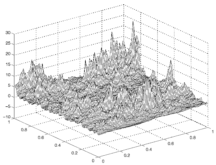
Recall that $S$ stands for the saturation of water. Denote by $I$ the identity matrix in $\mathbf{R}^{2\times 2}$, and assume the relative permeability tensor ${\mathcal{K}}(x)={k}(x)I$. Geostatistical models often suggest that the logarithm of the permeability field $k(x)$ is weakly or second order stationary in space, so that the mean log permeability is constant and its covariance only depends on the relative distance of two points rather than their actual location 1, 10, 11, 21 and 31. This is to say that the permeability field is generically a log-normal random field. In this section, we will test the performance of our mixed multiscale finite element method for a random log-normal permeability field. Here we generate the random log-normal permeability field ${k}(x)$ by using the moving ellipse average technique 10 with the variance of the logarithm of the permeability $\sigma ^2=1$, and the correlation lengths $l_1=0.3$ and $l_2=0.01$ in the $x_1$ and $x_2$ directions, respectively. One realization of the resulting permeability field in our numerical experiments is depicted in Figure 2.

Throughout we are interested in the fractional flow curves. A fractional flow curve $F(t)$ at time $t$ is defined as the production rate on $\Gamma _{\text{out}}$ by the following formula:

$$\begin{equation*} F(t)=\Big (\int ^1_0\ v_1(1,x_2,t)(1-S(1,x_2,t))\ dx_2\Big )\Big / \Big (\int ^1_0\ v_1(1,x_2,t)\ dx_2\Big ). \end{equation*}$$

Here $1-S$ stands for the saturation of the produced fluid (e.g., oil), and thus $F(t)$ represents the percentage of the produced oil over water. We also use the dimensionless time PVI in our computations. One PVI is the time required to fill the whole reservoir by injecting water at $\Gamma _{\text{in}}$. It is equal to 12

$$\begin{equation*} PVI=\frac{tv_1^{\text{average}}L_2}{L_1L_2} =tv_1^{\text{average}}, \end{equation*}$$

where $L_1$ and $L_2$ are the lengths of the cross-section of the reservoir in the $x_1$ and $x_2$ directions ($L_1,L_2$ are scaled to be $1$ in our simulations), $t$ is the real time and $v_1^{\text{average}}$ is the average velocity on $\Gamma _{\text{in}}$ in the $x_1$ direction. It is clear that in the unit of PVI, the time now is equal to the fraction of the water left in the whole reservoir, due to the heterogeneities of the medium.

The saturation equation 1.2 will be solved by an upwinding scheme in the finite element formulation; see 22 and 8. Given the discrete velocity field $\mathbf{v}_h$, for any $K\in \mathcal{M}_h$ with unit outer normal $\boldsymbol{\nu }$, we divide its boundary $\partial K$ into two parts:

$$\begin{eqnarray*} & &\partial K_-=\bigcup \ \{\ e\subset \partial K:\ \mathbf{v}_h(x_e)\cdot \boldsymbol{\nu }< 0\}, \quad \text{ inflow},\\ & &\partial K_+=\bigcup \ \{\ e\subset \partial K:\ \mathbf{v}_h(x_e)\cdot \boldsymbol{\nu }\ge 0\}, \quad \text{ outflow}. \end{eqnarray*}$$

Here $x_e$ is the midpoint of the side $e$. For any piecewise constant function $\eta _h$ over the mesh $\mathcal{M}_h$, we define its upwinding value on $\partial K$ as

$$\begin{eqnarray*} \tilde{\eta }_h=\left\{\begin{array}{ll} \eta _h^+\text{ (interior trace of $\eta _h$) } & \text{ on }\partial K_+,\\\eta _h^-\text{ (exterior trace of $\eta _h$) } & \text{ on }\partial K_-, \end{array}\right. \end{eqnarray*}$$

and assume $\eta _h^-=1$ on $\partial K_-\cap \Gamma _{\text{in}}.$ Let $\tau$ be the time step and $t^n=n\tau ,n\ge 1$. Then, denoting by $S^n_K$ the approximation of the water saturation in $K$ at time $t^n$, we use the following upwinding scheme to solve 1.2:

$$\begin{eqnarray} \frac{S^{n+1}_K-S^n_K}{\tau }+\int _{\partial K}\ (\mathbf{v}_h\cdot \boldsymbol{\nu })\tilde{S}^n_K\ ds=0\ \ \ \forall K\in \mathcal{M}_h. {\tag{5.1}} \end{eqnarray}$$

We note that in the scheme 5.1 only the normal components of the discrete velocity on the sides of each element $K$ are required. For the mixed finite element methods solving 1.1, such normal components are directly computed as part of the method. In the following simulations, the “exact” fractional flow curve is referred to the one computed by solving 1.1 by the lowest order Raviart-Thomas finite element method and 1.2 by the scheme 5.1 on the fine $1024\times 1024$ mesh.

Our first experiment in this subsection is designed to show the importance of the local conservation property in the flow transport simulations. Let $\mathbf{v}_h$ be the approximation of the Darcy velocity $\mathbf{v}=-{k}(x)\nabla p$; then the local conservation property means

$$\begin{eqnarray} \int _{\partial K}\ (\mathbf{v}_h\cdot \boldsymbol{\nu })\ ds=0\ \ \ \ \forall K\in \mathcal{M}_h. {\tag{5.2}} \end{eqnarray}$$

This is an important property, because if it is violated it would introduce unphysical numerical sources or sinks. It is clear that 5.2 is always satisfied when the mixed finite element method is used to solve 1.1. In this experiment we first solve the pressure equation 1.1 by using a standard conforming linear finite element method on the $1024\times 1024$ mesh to get $p_h$, and then we recover the normal components of the velocity by two different methods. For any $K\in \mathcal{M}_h$, in the first method we take $\mathbf{v}_h\cdot \boldsymbol{\nu }|_{\partial K}$ as the interior trace of $\mathbf{v}_h=-{k}(x)\nabla p_h$. The resulting fractional flow curve is depicted in Figure 3(a). We note that in this method the normal components of the velocity are in general discontinuous across the interelement boundaries, but the local conservation property 5.2 is satisfied since $k(x)$ is constant on each element $K$ and so is $\nabla p_h$. In the second method, we take $\mathbf{v}_h\cdot \boldsymbol{\nu }$ on any side $e\subset \partial K$ as the average of its values in two adjacent elements. The resulting fractional flow curve is shown in Figure 3(b). We can see clearly that the fractional flow curve obtained from the second method deviates significantly from the solid line obtained from the “exact” solution. Note that in this method the normal components are continuous across the interelement boundaries, but the local conservation property is violated. This shows that the local conservation property is more important than the continuity of the normal components. Moreover, we observe that the fractional flow curve computed by the first method is in good agreement with the “exact” one obtained by using the mixed method on the fine $1024\times 1024$ mesh. We remark that the mixed finite element method involves the computation of the solution of a discrete problem which has many more degrees of freedom than solving the pressure equation 1.1 using a linear finite element method. Thus, when one can afford to solve the whole system 1.1-1.2 on a fine mesh, instead of using the mixed finite element method, one should use the linear finite element method to solve the pressure equation 1.1 and then generate the velocity field by the first method mentioned above. However, we remark that the linear finite element method is a special case. If one uses higher order displacement finite element methods to solve 1.1, there are no obvious ways to recover the velocity field such that the local conservation property 5.2 is satisfied.

Next we compare the performance of the mixed multiscale finite element method and the displacement multiscale finite element method 18. One important feature of the multiscale finite element method is its ability to reconstruct locally the fine-scale velocity field from the coarse grid pressure solver. The key idea is to use the multiscale base functions to interpolate the fine grid solution. To demonstrate that we can accurately capture the correct small-scale velocity field, we first solve the pressure equation 1.1 on a coarse $64\times 64$ mesh and use the multiscale finite element basis functions to reconstruct the velocity field on the fine $1024\times 1024$ mesh. We then use this locally reconstructed fine grid velocity field to solve the saturation equation 1.2 on the fine $1024\times 1024$ mesh. In Figure 4(a), the resulting fractional flow curve is compared with the “exact” fractional flow curve which is obtained by solving the pressure and the saturation equations on the fine $1024\times 1024$ mesh using the mixed finite element method. As we can see from Figure 4(a), the two fractional flow curves agree very well.

We then solve the pressure equation 1.1 by the displacement over-sampling multiscale finite element method on a coarse $64\times 64$ mesh and use the displacement multiscale finite element bases to reconstruct the velocity field on the fine mesh. Again the saturation equation 1.2 is solved on the fine $1024\times 1024$ mesh. The resulting fractional flow curve and the “exact” fraction curve are shown in Figure 4(b). Due to the violation of the local conservation property, the displacement multiscale finite element method begins to deviate significantly from the “exact” fractional flow curve after some time (beyond $t=0.6$). This numerical example demonstrates that the over-sampling mixed multiscale finite element method provides a better way to locally reconstruct the fine grid velocity field which is suitable for long-time computations of the saturation field. This is an important consideration from a practical viewpoint.

5.3. The core-plug model: a coarse mesh algorithm

Now we describe how the proposed mixed multiscale finite element can be combined with the existing upscaling technique for the saturation equation 1.2 to get a complete coarse grid algorithm for the problem 1.1-1.2. The numerical upscaling of the saturation equation has been under intensive study in the literature, see 11, 14, 12, and 21. Here, we use the upscaling method proposed in 14 and 12 to design an overall coarse grid model for the problem 1.1-1.2. The work of 14 for upscaling the saturation equation involves a moment closure argument. The velocity and the saturation are separated into a local mean quantity and a small-scale perturbation with zero mean. For example, the Darcy velocity is expressed as $\mathbf{v}= \mathbf{v}_0+\mathbf{v}'$ in 1.2, where $\mathbf{v}_0$ is the average of the velocity $\mathbf{v}$ over each coarse element and $\mathbf{v}'=(\mathbf{v}'_1,\mathbf{v}'_2)$ is the deviation of the fine-scale velocity from its coarse-scale average. After some manipulations, an average equation for the saturation $S$ can be derived as follows 14:

$$\begin{eqnarray} \frac{\partial S}{\partial t}+\mathbf{v}_0\cdot \nabla S=\frac{\partial }{\partial x_i}\Big (D_{ij}(x,t) \frac{\partial S}{\partial x_j}\Big ), {\tag{5.3}} \end{eqnarray}$$

where the diffusion coefficients $D_{ij}(x,t)$ are defined by

$$\begin{equation*} D_{ii}(x,t)=\langle |\mathbf{v}'_i(x)|\rangle L^0_i(x,t),\ \ \ D_{ij}(x,t)=0,\ \ \text{for }i\not =j, \end{equation*}$$

$\langle |\mathbf{v}'_i(x)|\rangle$ stands for the average of $|\mathbf{v}'_i(x)|$ over each coarse element and $L^0_i(x,t)$ is the length of the coarse grid streamline in the $x_i$ direction which starts at time $t$ at point $x$, i.e.,

$$\begin{equation*} L_i^0(x,t)=\int ^t_0\ y_i(s)\ ds, \end{equation*}$$

where $y(s)$ is the solution of the following system of ODEs:

$$\begin{equation*} \frac{d y(s)}{ds}=\mathbf{v}_0(y(s)),\ \ \ y(t)=x. \end{equation*}$$

Note that the hyperbolic equation 1.2 is now replaced by a convection-diffusion equation. The convection-dominant parabolic equation 5.3 is solved by the characteristic linear finite element method 9, 26 in our simulation. The flow transport model 1.1-1.2 is solved in the coarse grid as follows:

1.

Solve the pressure equation 1.1 by the over-sampling mixed multiscale finite element method and obtain the fine-scale velocity field using the multiscale basis functions.

2.

Compute the coarse grid average $\mathbf{v}_0$ and the fine-scale deviation $\langle |\mathbf{v}'_i(x)|\rangle$ on the coarse grid.

3.

At each time step, solve the convection-diffusion equation 5.3 by the characteristic linear finite element method on the coarse grid in which the lengths $L_i^0(x,t)$ of the streamline are computed for the center of each coarse grid element.

The mixed multiscale finite element method can be readily combined with the above upscaling model for the saturation equation. The local fine grid velocity ${\mathbf{v}}'$ will be constructed from the multiscale finite element base functions. The main cost in the above algorithm lies in the computation of multiscale bases, which can be done a priori and completely in parallel. This algorithm is particularly attractive when multiple simulations must be carried out due to the change of boundary and source distribution, as is often the case in engineering applications. In such situation, the cost of computing the multiscale base functions is just overhead. Moreover, once these base functions are computed, they can be used for subsequent time integration of the saturation. Because the evolution equation is now solved on a coarse grid, a larger time step can be used. This also offers additional computational saving. For many oil recovery problems, due to the excessively large fine grid data, upscaling is a necessary step before performing many simulations and realizations on the upscaled coarse grid model. If one can coarsen the fine grid by a factor of 10 in each dimension, the computational saving of the coarse grid model over the original fine model could be as large as a factor 10,000 (three space dimensions plus time).

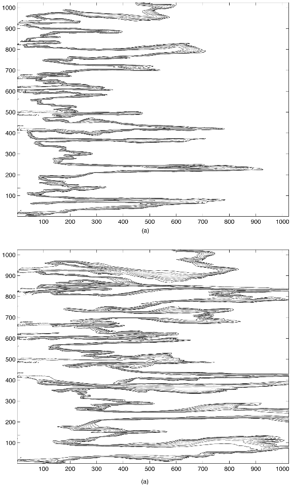
We perform a coarse grid computation of the above algorithm on the coarse $64\times 64$ mesh. The fractional flow curve using the above algorithm is depicted in Figure 5. It gives excellent agreement with the “exact” fractional flow curve. The contour plots of the saturation $S$ at times $t=0.25$ and $t=0.5$ are depicted in Figure 6. The contour plots of the saturation $S$ on the fine $1024\times 1024$ mesh at times $t=0.25$ and $t=0.5$ computed by using the “exact” velocity field are displayed in Figure 7. We observe that the contour plots in Figure 6 approximate the “exact” ones in Figure 7 in accuracy, but the sharp oil/water interfaces in Figure 7 are smeared out. This is due to the parabolic nature of the upscaled equation 5.3. We have also performed many other numerical experiments to test the robustness of this combined coarse grid model. We found that for permeability fields with strong layered structure, the above coarse grid model is very robust. The agreement with the fine grid calculations is very good. We are currently working towards a qualitative and quantitative understanding of this upscaling model. It is likely that one can justify this upscaling model for a periodic layered permeability field.

Finally, we remark that the upscaling equation 5.3 uses small-scale information $\mathbf{v}'$ of the velocity field to define the diffusion coefficients. This information can be constructed locally through the mixed multiscale basis functions. This is an important property of our multiscale finite element method. It is clear that solving directly the homogenized pressure equation

$$\begin{equation*} \operatorname {div}({\mathcal{K}}^*(x)\nabla p^*)=0 \end{equation*}$$

will not provide such small-scale information. On the other hand, whenever one can afford to resolve all the small-scale features by a fine grid, one can use fast linear solvers, such as multigrid methods, to solve the pressure equation 1.1 on the fine mesh. From the fine grid computation, one can easily construct the average velocity $\mathbf{v}_0$ and its deviation $\mathbf{v}'$. However, when multiple simulations must be carried out due to the change of boundary conditions, the pressure equation 1.1 will then have to be solved again on the fine mesh. The multiscale finite element method only solves the pressure equation once on a coarse mesh, and the fine grid velocity can be constructed locally through the finite element bases. This is the main advantage of our mixed multiscale finite element method. This process becomes more difficult for a nonlinear two-phase flow, due to the dynamic coupling between the pressure and the saturation. We are now investigating the possibility of upscaling the two-phase flow by using multiscale finite element base functions that are constructed from the one-phase flow (time-independent). In this case, we need to provide corrections to the pressure equation to account for the scale interaction near the oil/water interface.

Acknowledgments

We wish to thank Dr. Yalchin R. Efendiev for many inspiring discussions and for providing us the code generating the log-normal permeability field. We would also like to thank Dr. Hector Ceniceros for his valuable comments on our original manuscript, and the referee for his careful reading and constructive comments.

Figure 1.

The element $K$ and its over-sampling element $S(K)$: lower right elements (left) and upper right elements (right). The length of the horizontal and vertical edges of $S(K)$ is four times the corresponding length of the edges of $K$.

Table 1.

Results for the over-sampling method $\varepsilon /h=0.5$ and $N=32$.

M	$\varepsilon$	$\operatorname {RE}_1$	rate	$\operatorname {RE}_2$	rate
8	1/16	12.6155E-2		11.4035E-2
16	1/32	7.3081E-2	0.7870	6.5842E-2	0.7920
32	1/64	4.6645E-2	0.6478	4.1563E-2	0.6637
64	1/128	3.6665E-2	0.3473	2.5297E-2	0.7163

Table 2.

Results for the over-sampling method ($\varepsilon =1/128=0.0078125$).

Mesh
N	M	$\operatorname {RE}_1$	rate	$\operatorname {RE}_2$	rate
128	16	6.6152E-2		6.0833E-2
64	32	4.2149E-2	0.6503	3.4530E-2	0.8170
32	64	3.6664E-2	0.2011	2.5297E-2	0.4489
16	128	5.1504E-2	-0.4903	2.8311E-2	-0.1624

Figure 2.

The random log-normal permeability field ${k}(x)$. The ratio of maximum to minimum is $168.65$.

Figure 3.

Comparison of two different methods recovering the normal components of the velocity from piecewise linear pressure $p_h$. Each solid line is the “exact” fractional flow curve using the mixed finite element method solving the pressure equation. (a) The dotted line is the fractional flow curve obtained from the first method of local velocity recovery, which satisfies the local conservation property. (b) The dotted line is the fractional flow curve obtained from the second method of local velocity recovery, which violates the local conservation property.

Figure 4.

Comparison of the mixed multiscale finite element method and the displacement multiscale finite element method. Each solid line is the “exact” fractional flow curve using the mixed finite element method to solve the pressure equation. (a) The dotted line is the fractional flow curve using the velocity by the mixed multiscale finite element method. (b) The dotted line is the fractional flow curve using the velocity recovered from the displacement multiscale finite element method.

Figure 5.

The accuracy of the coarse grid algorithm. The solid line is the “exact” fractional flow curve using the mixed finite element method for solving the pressure equation. The slash-dotted line is the fractional flow curve using the above coarse grid algorithm.

Figure 6.

The contour plots of the saturation $S$ computed using the upscaled model on a $64\times 64$ mesh at time $t=0.25$ (left) and $t=0.5$ (right)

Figure 7.

The contour plots of the saturation $S$ computed on the fine $1024\times 1024$ mesh using the “exact” velocity field at time $t=0.25$ (left) and $t=0.5$ (right)