The Image Deblurring Problem: Matrices, Wavelets, and Multilevel Methods

1. Introduction

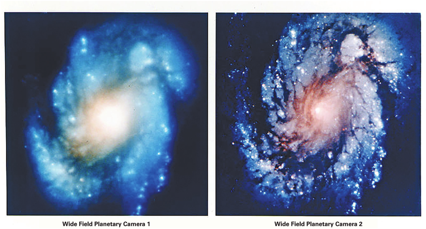
After the launch of the Hubble Space Telescope in 1990, astronomers were gravely disappointed by the quality of the images as they began to arrive. Due to miscalibrated testing equipment, the telescope’s primary mirror had been ground to a shape that differed slightly from the one intended, resulting in the misdirection of incoming light as it moved through the optical system. The blurry images did little to justify the telescope’s $1.5 billion price tag 1. Three years later, space shuttle astronauts installed a specially designed corrective optical system that essentially fixed the problem and yielded spectacular images (See the image on this page. Hubble’s view of the M100 galaxy soon after launch is on the left and on the right is the view after corrective optics were installed in 1993). In the meantime, mathematicians devised several ways to convert the blurry images into high-quality images. The process of mathematical deblurring is the focus of this article.

Blurred images can be caused by many factors such as the movement of the imaging device or the target object, focus errors, or the presence of atmospheric turbulence 12. Indeed, the need for image deblurring goes beyond Hubble’s story. For instance, the image deblurring problem is encountered in many applications such as pattern recognition, computer vision, and machine intelligence. Moreover, image deblurring shares the same mathematical formulation as other imaging modalities. For instance, in many cases we have only limited opportunities to capture an image; this is particularly true of medical images, such as computerized tomography (CT), proton computed tomography (pCT), and magnetic resonance imaging (MRI), for which equipment and patient availability are scarce resources. In cases such as these, we need a way to extract meaningful information from noisy images that have been collected during the data acquisition process.

In this article, we will describe a mathematical model of how digital images become blurry as well as several mathematical issues that arise when we try to undo the blurring. While blurring may be effectively modeled by a linear process, we will see that deblurring is not as simple as inverting that linear process. Indeed, deblurring belongs to an important class of problems known as discrete ill-posed problems 10, and we will introduce some techniques that have become standard for solving them. In addition, we will describe some matrix structures in the linear operators that will allow more efficient computations.

2. Digital Images and Blurring

We start by describing digital images and a process by which they become blurry. As illustrated in Figure 1, the lens of a digital camera directs photons entering the camera onto a charge-coupled device (CCD), which consists of a rectangular $p\times q$ array of detectors. Each detector in the CCD converts a count of the photons into an electrical signal that is digitized by an analog-to-digital converter (ADC). The result is a digital image stored as a $p\times q$ matrix whose entries represent the intensities of light recorded by each of the CCD’s detectors.

Figure 1.

A simple model of how a digital image is created.

A grayscale image is represented by a single matrix with integer entries describing the brightness at each location. A color image is represented by three matrices that describe the colors in terms of their red, green, and blue constituents. Of course, we may see these matrices by zooming in on a digital image until we see individual pixels, picture elements that contain only one intensity value.

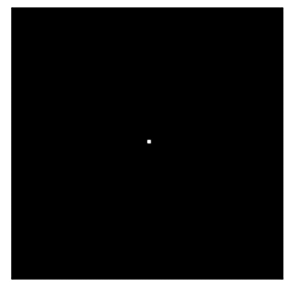
Perhaps due to imperfections in the camera’s lens or the lens being improperly focused, it is inevitable that photons intended for one pixel bleed over into adjacent pixels, and this leads to blurring of the image. To illustrate, we will consider grayscale images comprised of arrays of $64\times 64$ pixels. In Figure 2, the image on the left shows a single pixel illuminated while on the right we see how photons intended for this single pixel have spilled over into adjacent pixels to create a blurred image.

Figure 2.

The intensity from a single pixel, shown on the left, is spread out across adjacent pixels according to a Gaussian blur, as seen on the right.

There are several models used to describe blurring. A simple one that we choose here has the light intensity contained in a single pixel $(i, j)$ spilling over into an adjacent pixel $(k, l)$ according to the Gaussian point spread function

$$\begin{equation} \frac{1}{N}\exp \left(-\frac{1}{2}\left(\frac{k-i}{s}\right)^2 - \frac{1}{2}\left(\frac{l-j}{s}\right)^2\right) = \frac{1}{N}\exp \left(-\frac{1}{2}\left(\frac{k-i}{s}\right)^2\right) \exp \left(-\frac{1}{2}\left(\frac{l-j}{s}\right)^2\right), \tag{1}{} \end{equation}$$

where $s$ is a parameter that controls the spread in the intensity and $N$ is a normalization constant so that the total intensity sums to 1. As we will see later, the fact that the two-dimensional Gaussian can be written as a product of one-dimensional Gaussians has important consequences for our ability to efficiently represent the blurring process as a linear operator.

Though we visually experience a grayscale image as a $p\times q$ matrix of pixels $\mathbf{X}$, we will mathematically represent an image as a $pq$-dimensional vector $\mathbf{x}$ by stacking the columns of $\mathbf{X}$ on top of one another. That is, $\mathbf{x}= {\mathrm{v}ec}(\mathbf{X}) = (\mathbf{X}_{11},\ldots ,\mathbf{X}_{p1},\mathbf{X}_{12},\ldots ,\mathbf{X}_{p2},\ldots , \mathbf{X}_{1q},\ldots ,\mathbf{X}_{pq})^T$ with $\mathbf{X}_{ij}$ being the intensity value of the pixel at row $i$ and column $j$. The blurring process is linear as the number of photons that arrive at one pixel is the sum of the number of misdirected photons intended for nearby pixels. Therefore, if $\mathbf{B}$ is the blurred image represented by the vector $\mathbf{b}={\mathrm{v}ec}(\mathbf{B})$, then there is a blurring matrix $\mathbf{A}$ that blurs the original image $\mathbf{x}$ into the blurred image $\mathbf{b}= \mathbf{A}\mathbf{x}$. Furthermore, we assume that both images $\mathbf{X}$ and $\mathbf{B}$ have the same size, as do $\mathbf{x}$ and $\mathbf{b}$, which implies that the matrix $\mathbf{A}$ is square. Deblurring refers to the inverse process of recovering the original image $\mathbf{x}$ from its blurred counterpart $\mathbf{b}$ and includes situations, unlike the one we describe here, where $\mathbf{A}$ is not invertible or even square.

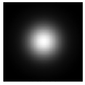
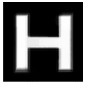
Each column of $\mathbf{A}$ is the result of blurring a single pixel, which means that each column of $\mathbf{A}$ represents the point spread function centered at its corresponding pixel $(i,j)$. When that center is near the edge of the image, some photons will necessarily be lost outside the image, and there are a few options for how to incorporate this fact into our model. In real-life settings, it is possible to have knowledge only over a finite region, the so called Field of View (FOV), that defines the range that a user can see from an object. It is then necessary to make an assumption on what is outside the FOV by means of the boundary conditions. For instance, one option to overcome the loss outside the FOV is to simply accept that loss, in which case we say that the matrix has zero boundary conditions. This has the effect of assuming that the image is black (pixel values are zero) outside the FOV, which can lead to an artificial black border around a deblurred image (see the image on the left on Figure 3⁠¹).

¹

We picked the letter H to celebrate Hispanic Heritage Month, which is the focus of this issue of Notices.

✖

In some contexts, it can be advantageous to impose reflexive boundary conditions, which assume that the photons are reflected back onto the image. In other scenarios of interest, periodic boundary conditions, which assume the lost photons reappear on the opposite side of the image as if the image repeats itself indefinitely in all directions outside the FOV, are a suitable fit. Nevertheless, in practical settings, we periodically extend only some pixel values close to the boundary (see the image on the right on Figure 3).

Figure 3.

Image with assumed zero boundary conditions is shown on the left and one with assumed periodic boundary condition is shown on the right. The red box represents the FOV.

3. Adding Noise

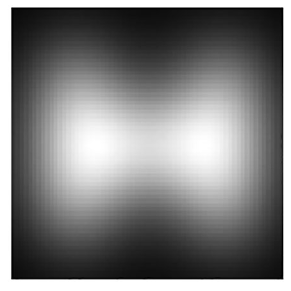
Let us consider the grayscale image $\mathbf{x}^{\mathrm{true}}$ shown on the left of Figure 4 and its blurred version $\mathbf{b}^{\mathrm{true}} = \mathbf{A}\mathbf{x}^{\mathrm{true}}$ shown on the right.

Figure 4.

An image $\mathbf{x}^{\mathrm{true}}$ on the left is blurred to obtain $\mathbf{b}^{\mathrm{true}}$ on the right.

If we had access to $\mathbf{b}^{\mathrm{true}}$, it would be easy enough to recover $\mathbf{x}^{\mathrm{true}}$ by simply solving the linear system $\mathbf{A}\mathbf{x}= \mathbf{b}^{\mathrm{true}}$ since our model gives a square, invertible matrix $\mathbf{A}$. However, the conversion of photon counts into an electrical signal by the CCD and then a digital reading by the ADC introduces electrical noise into the image that is ultimately recorded. The recorded image $\mathbf{b}$ is therefore a noisy approximation of the true blurred image $\mathbf{b}^{\mathrm{true}}$, so we write $\mathbf{b}= \mathbf{b}^{\mathrm{t}rue}+\mathbf{e}$, where $\mathbf{e}$ is a noise vector whose entries are independent and identically distributed random variables. There are various models used to describe the kind of noise added. For instance, we might assume that the noise is Gaussian white noise, which means that the entries in $\mathbf{e}$ are sampled from a normal distribution with mean zero. In our example, we assume that $\|\mathbf{e}\|_2 = 0.001\|\mathbf{b}^{\mathrm{true}}\|_2$, that is, the white noise is about 0.1% of the image $\mathbf{b}^{\mathrm{true}}$. As seen in Figure 5, this level of noise cannot be easily detected.

Figure 5.

The blurred image $\mathbf{b}^{\mathrm{true}}$ on the left with a small amount of Gaussian white noise added to obtain $\mathbf{b}$ on the right.

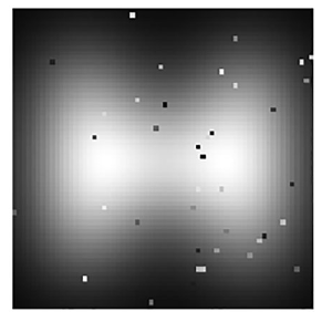
Two other models of noise are illustrated in Figure 6. The image on the left contains what is called Poisson noise. Under low light conditions, as encountered in astronomical imaging, the number of photons that arrive on the CCD are very low and therefore the noise produced is better modeled by a Poisson distribution than a Gaussian one 19. If the digital image is transmitted over a communication channel, some of the transmitted bits may be corrupted in transmission, resulting in “salt and pepper” noise, the effect of which is shown in the image to the right 12. This noise can be modeled by a uniform distribution whose standard deviation is inversely proportional to the number of bits used. In the rest of the article, we will assume that we have Gaussian white noise. Some references on how to model and solve other noise models are included in 20.

Figure 6.

Poisson noise is added to the blurred image on the left and salt and pepper noise on the right.

Because our recorded image $\mathbf{b}$ is a good approximation of $\mathbf{b}^{\mathrm{true}}$, we might naïvely expect to find a good approximation of $\mathbf{x}^{\mathrm{true}}$ by solving the linear system of equations $\mathbf{A}\mathbf{x}= \mathbf{b}$. However, its solution, which we call $\mathbf{x}^{LS}$, turns out to be very different from the original image $\mathbf{x}^{\mathrm{true}}$ as is seen in Figure 7. As we will soon see, this behavior results from the fact that deblurring is a discrete linear ill-posed problem.

Figure 7.

On the left we see the original image $\mathbf{x}^{\mathrm{true}}$ while the right shows $\mathbf{x}^{LS}$, the solution to the equation $\mathbf{A}\mathbf{x}= \mathbf{b}$, where $\mathbf{b}$ is the noisy recorded image.

We are now faced with two questions: how can we reconstruct the original image $\mathbf{x}^{\mathrm{true}}$ more faithfully and how can we do it in a computationally efficient way. For instance, today’s typical phone photos have around 10 million pixels, which means that the number of entries in the blurring matrix $\mathbf{A}$ is about 100 trillion. Working with a matrix of that size will require some careful thought.

4. Discrete Linear Ill-Posed Problems

The singular value decomposition (SVD) of the matrix $\mathbf{A}$ offers insight into why the naïvely reconstructed image $\mathbf{x}^{LS}$ differs so greatly from the original $\mathbf{x}^{\mathrm{true}}$. Consider both vectors $\mathbf{x}^{\mathrm{true}}$ and $\mathbf{b}$ of dimension $m=pq$. Now suppose that $\mathbf{A}\in \mathbb{R}^{m\times m}$ has full rank and its SVD is given by

$$\mathbf{A}= \mathbf{U}\boldsymbol{\Sigma }\mathbf{V}^T = \sum _{\ell =1}^m \sigma _\ell \mathbf{u}_\ell \mathbf{v}_\ell ^T,$$

where $\mathbf{U}=(\mathbf{u}_1,\ldots ,\mathbf{u}_m)\in \mathbb{R}^{m\times m}$ and $\mathbf{V}=(\mathbf{v}_1,\ldots ,\mathbf{v}_m)\in \mathbb{R}^{m\times m}$ are matrices having orthonormal columns so that $\mathbf{U}^T\mathbf{U}= \mathbf{V}^T\mathbf{V}=\mathbf{I}$, and $\boldsymbol{\Sigma }= {\mathrm{d}iag}(\sigma _1,\ldots ,\sigma _m)$, with $\sigma _1\geq \sigma _2\geq \ldots \geq \sigma _m > 0$, that is to say, $\boldsymbol{\Sigma }$ is an $m\times m$ diagonal matrix, whose entries are positive and appear in decreasing order. The scalars $\sigma _\ell$ are the singular values of $\mathbf{A}$ and the vectors $\mathbf{u}_\ell$ and $\mathbf{v}_\ell$ are the left and right singular vectors of $\mathbf{A}$, respectively. In particular, the singular value decomposition provides orthonormal bases defined by the columns of $\mathbf{U}$ and $\mathbf{V}$, for the range and domain spaces, respectively, so that $\mathbf{A}\mathbf{v}_\ell = \sigma _\ell \mathbf{u}_\ell$. Notice that we are assuming that the matrix $\mathbf{A}$ is square and full rank, since all the singular values are positive, and therefore invertible. This is natural in the image deblurring model described here. In other inverse problems, however, the matrix $\mathbf{A}$ may be square but rank-deficient or even rectangular, situations whose solutions require more detailed considerations 10.

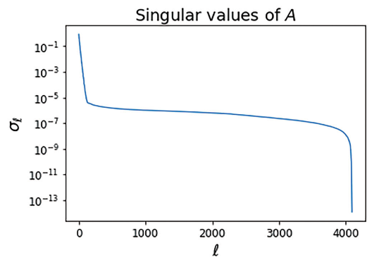
Discrete linear ill-posed problems are characterized by three properties, which are satisfied by the deblurring problem. First, the singular values $\sigma _\ell$ decrease to zero without a large gap separating a group of large singular values from a group of smaller ones. The plot of the singular values in Figure 8 shows that the difference between the largest and smallest singular values is about thirteen orders of magnitude, which indicates that $\mathbf{A}$ is highly ill-conditioned.

Figure 8.

The singular values $\sigma _\ell$ of $\mathbf{A}$.

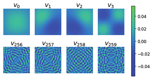
Second, the singular vectors $\mathbf{u}_\ell$ and $\mathbf{v}_\ell$ become more and more oscillatory as $\ell$ increases. Figure 9 shows images $\mathbf{V}_\ell$ representing eight right singular vectors $\mathbf{v}_\ell$ ($\mathbf{v}_\ell ={\mathrm{v}ec}(\mathbf{V}_\ell )$) of the blurring matrix constructed above and demonstrates how the frequency of the oscillations increases as $\ell$ increases. Since the blurring matrix $\mathbf{A}$ spreads out any peaks in an image, it tends to dampen high-frequency oscillations. Therefore, a right singular vector $\mathbf{v}_\ell$ representing a high frequency will correspond to a small singular value $\sigma _\ell$ since $\mathbf{A}\mathbf{v}_\ell = \sigma _\ell \mathbf{u}_\ell$. This oscillatory behavior of the singular vectors and their relation to the singular values appears more generally with other blurring operators defined by other kernels and in other discrete ill-posed inverse problems due to the underlying continuous model 10.

Figure 9.

Images corresponding to eight right singular vectors $\mathbf{v}_\ell$.

The third property of discrete linear ill-posed problems is known as the discrete Picard condition, which says that the coefficients of $\mathbf{b}^{\mathrm{true}}$ expressed in the left singular basis, $|\mathbf{u}_\ell ^T\mathbf{b}^{\mathrm{true}}|$, on average, decay to zero faster than the singular values $\sigma _\ell$ 10. This is illustrated on the top of Figure 10, which shows both $|\mathbf{u}_\ell ^T\mathbf{b}^{\mathrm{true}}|$ and the singular values $\sigma _\ell$. Since $\mathbf{u}_\ell ^T\mathbf{b}^{\mathrm{true}}=\sigma _\ell \mathbf{v}_\ell ^T\mathbf{x}^{\mathrm{true}}$, the discrete Picard condition holds when the original image $\mathbf{x}^{\mathrm{true}}$ is not dominated by high-frequency contributions $\mathbf{v}_\ell ^T\mathbf{x}^{\mathrm{true}}$ for large $\ell$. This is a reasonable assumption with most digital photographs 12.

Figure 10.

The coefficients $|\mathbf{u}_\ell ^T\mathbf{b}^{\mathrm{true}}|$ are seen on the top while the coefficients $|\mathbf{u}_\ell ^T\mathbf{b}|$ are on the bottom.

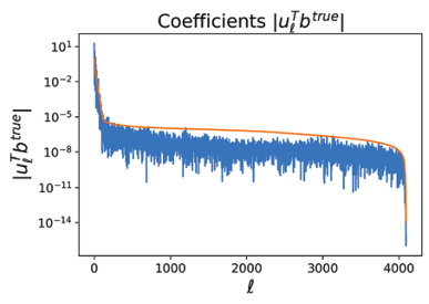
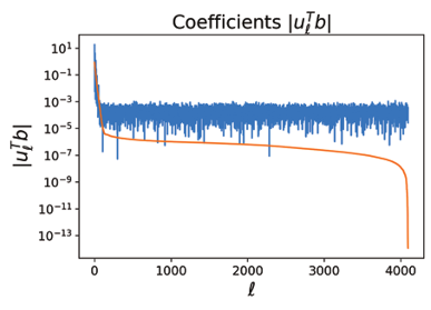
By contrast, the added white noise causes the coefficients $|\mathbf{u}_\ell ^T\mathbf{b}| = |\mathbf{u}_\ell ^T\mathbf{b}^{\mathrm{true}} + \mathbf{u}_\ell ^T\mathbf{e}|$ to remain relatively constant for large $\ell$, as can be seen on the bottom of Figure 10. However, both plots agree for small values of $\ell$.

Writing both vectors $\mathbf{x}^{LS}$ and $\mathbf{x}^{\mathrm{true}}$ as a linear combination of the right singular vectors $\mathbf{v}_\ell$, we see that

$$\mathbf{x}^{\mathrm{true}} = \sum _{\ell =1}^{m} \frac{\mathbf{u}_\ell ^T \mathbf{b}^{\mathrm{true}}}{\sigma _\ell } \mathbf{v}_\ell$$

and

$$\begin{aligned} \mathbf{x}^{LS}&= \sum _{\ell =1}^{m} \frac{\mathbf{u}_\ell ^T \mathbf{b}}{\sigma _\ell } \mathbf{v}_\ell =\sum _{\ell =1}^{m} \frac{\mathbf{u}_\ell ^T (\mathbf{b}^{\mathrm{true}}+\mathbf{e})}{\sigma _\ell } \mathbf{v}_\ell \\ &= \sum _{\ell =1}^{m} \frac{\mathbf{u}_\ell ^T \mathbf{b}^{\mathrm{true}}}{\sigma _\ell } \mathbf{v}_\ell + \sum _{\ell =1}^{m} \frac{\mathbf{u}_\ell ^T \mathbf{e}}{\sigma _\ell } \mathbf{v}_\ell \\ & = \mathbf{x}^{\mathrm{true}} + \sum _{\ell =1}^{m} \frac{\mathbf{u}_\ell ^T \mathbf{e}}{\sigma _\ell } \mathbf{v}_\ell . \end{aligned}$$

Because the singular values approach zero, the coefficients $|\mathbf{u}_\ell ^T\mathbf{e}|/\sigma _\ell$ grow extremely large, as seen in Figure 11. Therefore, $\mathbf{x}^{LS}$ includes a huge contribution from high-frequency right singular vectors $\mathbf{v}_\ell$, which means that $\mathbf{x}^{LS}$ is very oscillatory and not at all related to the original image $\mathbf{x}^{\mathrm{true}}$ that we seek to reconstruct.

Figure 11.

The coefficients of $\mathbf{x}^{\mathrm{true}}$ and $\mathbf{x}^{LS}$.

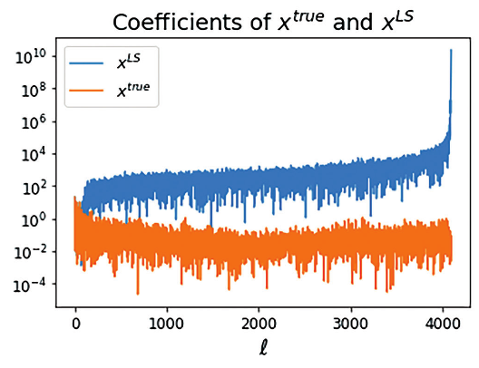
We also note here that the size of the coefficients shown in Figure 11 cause the norm $\|\mathbf{x}^{LS}\|_2$ to be extremely large. As we will see shortly, we will consider this norm as a measure of the amount of noise in the reconstructed image.

5. Regularization

As an alternative to accepting $\mathbf{x}^{LS}$ as our reconstructed image, we instead approximate $\mathbf{x}^{\mathrm{true}}$ by filtering out the contributions from the high-frequency singular vectors, which are magnified through division by small singular values, while retaining as much information as possible from the measured data $\mathbf{b}$. While we know the noise vector $\mathbf{e}$ in the example presented here, in practice we do not, which means we cannot expect to get rid of the noise completely. Therefore, the goal is to design filtering methods that dampen the effects of the noise given that very little is known about it. This process is known as regularization, and there are several possible approaches we can follow.

A first natural idea is to introduce a set of filtering factors $\phi _\ell$ on the SVD expansion and construct a regularized solution as

$$\mathbf{x}^{\mathrm{reg}} = \sum _{\ell =1}^{m} \phi _\ell \frac{\mathbf{u}_\ell ^T \mathbf{b}}{\sigma _\ell } \mathbf{v}_\ell ,$$

with the filter factors being $\phi _\ell \approx 0$ for large values of $\ell$ when the noise dominates and $\phi _\ell \approx 1$ for small values of $\ell$, which are the terms in the expansion where the components of $\mathbf{b}$ and $\mathbf{b}^{\mathrm{t}rue}$ are closest.

One option is to define $\phi _\ell =1$ for $\ell$ smaller than some cutoff $k<m$ and $\phi _\ell =0$ otherwise. That is, we can simply truncate the expansion of $\mathbf{x}^{LS}$ in terms of right singular vectors in an attempt to minimize the contribution from the terms $|\mathbf{u}_\ell ^T\mathbf{e}|/\sigma _\ell$ for large $\ell$. Then, the obtained regularized solution would be

$$\mathbf{x}^{\mathrm{T}SVD} = \sum _{\ell =1}^{k} \frac{\mathbf{u}_\ell ^T \mathbf{b}}{\sigma _\ell } \mathbf{v}_\ell .$$

This solution is known as the truncated SVD (TSVD).

Remember, however, that the singular values in discrete ill-posed problems approach zero without having a gap that would form a natural cutoff point. Instead, Tikhonov regularization chooses the filtering factors

$$\phi _\ell = \frac{\sigma _\ell ^2}{\sigma _\ell ^2 + \lambda ^2}$$

for some parameter $\lambda$ whose choice will be discussed later. For now, notice that $\phi _\ell \approx 1$ when $\sigma _\ell \gg \lambda$ and $\phi _\ell \approx 0$ when $\sigma _\ell \ll \lambda$. This has the effect of truncating the singular vector expansion at the point where the singular values pass through $\lambda$ but doing so more smoothly. Thus, the Tikhonov solution can be written as

$$\mathbf{x}^{\mathrm{T}ik} = \sum _{\ell =1}^{m} \frac{\sigma _\ell }{\sigma _\ell ^2 + \lambda ^2}(\mathbf{u}_\ell ^T \mathbf{b}) \mathbf{v}_\ell ,$$

which may also be rewritten as

$$\mathbf{x}^{\mathrm{T}ik} = (\mathbf{A}^T\mathbf{A}+\lambda ^2\mathbf{I})^{-1}\mathbf{A}^T\mathbf{b}.$$

This demonstrates that $\mathbf{x}^{\mathrm{T}ik}$ solves the least squares problem

$$\begin{equation} \mathbf{x}^{\mathrm{T}ik}=\operatorname *{argmin}_{\mathbf{x}} \{\|\mathbf{A}\mathbf{x}-\mathbf{b}\|_2^2 + \lambda ^2\|\mathbf{x}\|_2^2\},\tag{2}{} \end{equation}$$

where $\operatorname *{argmin}_{\mathbf{x}}\{f(\mathbf{x})\}$ returns the value of $\mathbf{x}$ which minimizes the function $f(\mathbf{x})$.

Equation 2 is a helpful reformulation of Tikhonov regularization. First, writing $\mathbf{x}^{\mathrm{T}ik}$ as the solution of a least squares problem provides us with efficient computational alternatives to finding the SVD of $\mathbf{A}$ 10. Moreover, the minimization problem provides insight into choosing the optimal value of the regularization parameter $\lambda$, as we will soon see.

By the way, this formulation of Tikhonov regularization shows its connection to ridge regression, a data science technique for tuning a linear regression model in the presence of multicollinearity to improve its predictive accuracy.

Let us investigate the meaning of 2. Notice that

$$\begin{equation} \|\mathbf{A}\mathbf{x}^{\mathrm{true}} - \mathbf{b}\|_2^2 = \|\mathbf{b}^{\mathrm{true}} - \mathbf{b}\|_2^2 = \|\mathbf{e}\|_2^2, \tag{3}{} \end{equation}$$

which is relatively small. We therefore consider the residual $\|\mathbf{A}\mathbf{x}-\mathbf{b}\|_2^2$ as a measure of how far away we are from the original image $\mathbf{x}^{\mathrm{true}}$. Remember that $|\mathbf{u}_\ell ^T\mathbf{e}|/\sigma _\ell$, the contributions to $\mathbf{x}^{LS}$ from the added noise, cause $\|\mathbf{x}^{LS}\|_2$ to be very large. Consequently, we think of the second term in 2 as measuring the amount of noise in $\mathbf{x}$.

The regularization parameter $\lambda$ allows us to balance these two sources of error. For instance, when $\lambda$ is small, the Tikhonov solution $\mathbf{x}^{\mathrm{T}ik}$, which is the minimum of 2, will have a small residual $\|\mathbf{A}\mathbf{x}^{\mathrm{T}ik}-\mathbf{b}\|_2$ at the expense of a large norm $\|\mathbf{x}^{\mathrm{T}ik}\|_2$. In other words, we tolerate a noisy regularized solution in exchange for a small residual. On the other hand, if $\lambda$ is large, the Tikhonov solution will have a relatively large residual in exchange for filtering out a lot of the noise.

6. Choosing the Regularizing Parameter $\lambda$

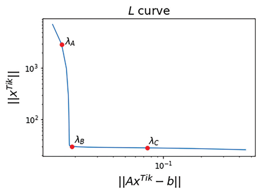
When applying Tikhonov regularization for solving discrete ill-posed inverse problems, a question of high interest is: How can we define the best regularization parameter $\lambda$? A common and well known technique is to create a log-log plot of the residual norm $\|\mathbf{A}\mathbf{x}^{\mathrm{T}ik}-\mathbf{b}\|_2$ and the solution norm $\|\mathbf{x}^{\mathrm{T}ik}\|_2$ as we vary $\lambda$. This plot, as shown in Figure 12, is usually called an $L$-curve due to its characteristic shape 13.

As mentioned earlier, small values of $\lambda$ lead to noisy regularized solutions while large values of $\lambda$ produce large residuals. This means that we move across the $L$-curve from the upper left to the lower right as we increase $\lambda$.

Figure 12.

The $L$-curve in our sample deblurring problem. The three indicated points correspond to values of $\lambda = \lambda _A, \lambda _B$, and $\lambda _C$.

Since the filtering factors satisfy $\phi _\ell \approx 1$ when $\sigma _\ell \gg \lambda$ and $\phi _\ell \approx 0$ when $\sigma _\ell \ll \lambda$, we will view the point where $\sigma _\ell = \lambda$ as an indication of where we begin filtering. Let us first consider the value $\lambda = \lambda _A$, which produces the point on the $L$-curve indicated in Figure 12. The resulting coefficients $|\mathbf{u}_\ell ^T\mathbf{b}|$ and $\phi _\ell |\mathbf{u}_\ell ^T\mathbf{b}|$ are shown in Figure 13. Filtering begins roughly where the plot of singular values crosses the horizontal line indicating the value of $\lambda _A$.

Figure 13.

The choice $\lambda =\lambda _{A}$ leads to under-smoothing.

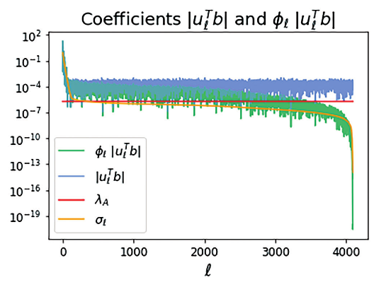
While we have filtered out some of the noise, it appears that there is still a considerable amount of noise present. This is reflected by the position of the corresponding point on the $L$-curve since the norm $\|\mathbf{x}^{\mathrm{T}ik}\|_2$ is relatively large. This choice of $\lambda$ is too low, and we say that the regularized solution is under-smoothed.

Alternatively, let us consider the regularized solution constructed with $\lambda = \lambda _C$ as indicated on Figure 12. This leads to the coefficients $|\mathbf{u}_\ell ^T\mathbf{b}|$ and $\phi _\ell |\mathbf{u}_\ell ^T\mathbf{b}|$ shown in Figure 14.

Figure 14.

The choice $\lambda =\lambda _C$ leads to over-smoothing.

In this case, we begin filtering too soon so that, while we have filtered the noise, we have also discarded some of the information present in $\mathbf{b}$, which is reflected in the relatively large residual $\|\mathbf{A}\mathbf{x}^{\mathrm{T}ik}-\mathbf{b}\|_2$. This choice of $\lambda$ is too large, and we say that the Tikhonov solution is over-smoothed.

Finally, considering the case where $\lambda = \lambda _B$ gives the Tikhonov solution that appears at the sharp bend of the $L$-curve in Figure 12. The resulting coefficients shown in Figure 15 inspire confidence that this is a good choice for $\lambda$.

Figure 15.

The choice $\lambda =\lambda _B$ gives the optimal amount of smoothing.

In this case, decreasing $\lambda$ causes us to move upward on the $L$-curve; we are allowing more high-frequency components into the solution without improving the residual. Increasing $\lambda$ causes us to move right on the $L$-curve; we are losing information as the residual increases without removing relevant high-frequency components. Therefore, $\lambda = \lambda _B$ is our optimal value.

Figure 16 shows the image $\mathbf{x}^{{\mathrm{T}ik}}$ obtained using this optimal parameter $\lambda =\lambda _B$. While it is not a perfect reconstruction of the original image $\mathbf{x}^{\mathrm{true}}$, it is a significant improvement over the recorded image $\mathbf{b}$. Accurately reproducing the sharp boundaries that occur in $\mathbf{x}^{\mathrm{true}}$ requires high-frequency contributions that we have necessarily filtered out.

Figure 16.

The reconstructed image $\mathbf{x}^{{\mathrm{T}ik}}$ using the regularization parameter determined by the $L$-curve is seen on the right, along with the original image $\mathbf{x}^{\mathrm{true}}$ on the left for comparison.

The $L$-curve furnishes a practical way to identify the optimal regularizing parameter as there are techniques that allow us to identify the point of maximal curvature by computing the Tikhonov solution for just a few choices of $\lambda$. However, this technique should not be applied uncritically as there are cases in which the optimal Tikhonov solution does not converge to the true image as the added error approaches zero.

An alternative technique, known as the Discrepancy Principle 6, relies on an estimate of the size of the error $\|\mathbf{e}\|_2$. Remember from 3 that we have $\|\mathbf{A}\mathbf{x}^{\mathrm{true}} - \mathbf{b}\|_2 = \|\mathbf{e}\|_2$. Moreover, the SVD description of $\mathbf{x}^{\mathrm{T}ik}$ provides a straightforward explanation for why the residual $\|\mathbf{A}\mathbf{x}^{\mathrm{T}ik} - \mathbf{b}\|_2$ is an increasing function of $\lambda$. If we know $\|\mathbf{e}\|_2$, we simply choose the optimal $\lambda$ to be the one where $\|\mathbf{A}\mathbf{x}^{\mathrm{T}ik} - \mathbf{b}\|_2 = \|\mathbf{e}\|_2$.

Other well-known methods for choosing the parameter $\lambda$ include the Generalized Cross Validation (GCV) 8, that chooses $\lambda$ to maximize the accuracy with which we can predict the value of a pixel that has been omitted, the unbiased predictive risk estimator (UPRE) 15, and more recently, methods based on learning when training data are available 4. Most of these methods can also be used to find the regularization parameter $k$ involved in the TSVD solution.

7. Other Regularization Techniques

Looking at the variational formulation 2 of Tikhonov regularization, it is easy to see how it can be extended to define other regularization methods by, for example, using different regularization terms.

7.1. General-form Tikhonov regularization

The Tikhonov regularization formulation 2 can be generalized to

$$\begin{equation} \min _{\mathbf{x}} \{\|\mathbf{A}\mathbf{x}- \mathbf{b}\|^2_2 + \lambda ^2\|\mathbf{L}\mathbf{x}\|^2_2\}, \tag{4}{} \end{equation}$$

by incorporating a matrix $\mathbf{L}$, which is called the regularization matrix 10. Its choice is problem dependent and can significantly affect the quality of the reconstructed solution. Several choices of the regularization matrix involve discretization of the derivative operators or framelet and wavelet transformations depending on the application. The only requirement on $\mathbf{L}$ is that it should satisfy

$$\begin{equation*} \mathcal{N}(\mathbf{A})\cap \mathcal{N}(\mathbf{L})=\{0\}, \end{equation*}$$

where $\mathcal{N}(\mathbf{M})$ denotes the null space of the matrix $\mathbf{M}$. The general Tikhonov minimization problem 4 has the unique solution

$$\begin{equation*} \mathbf{x}^{{\mathrm{G}Tik}}=(\mathbf{A}^T\mathbf{A}+\lambda ^2 \mathbf{L}^T\mathbf{L})^{-1}\mathbf{A}^T\mathbf{b} \end{equation*}$$

for any $\lambda >0$.

Figure 17.

The reconstructed images using the optimal regularization parameter and the discretization of the first derivative operator with the 2-norm regularization on the left, and TV regularization on the right.

In Figure 17, we reconstruct the image by applying the discretization of the two-dimensional first derivative operator for zero boundary conditions, that is, the matrix $\mathbf{L}$ takes the form of

$$\begin{equation} \mathbf{L}=\left( \begin{matrix} \mathbf{I}&\otimes &\mathbf{L}_1\\ \mathbf{L}_1&\otimes & \mathbf{I}\end{matrix}\right) \text{with } \mathbf{L}_1=\left( \begin{smallmatrix} -1 & 1&&&\\ &-1&1&&\\ &&\ddots &\ddots &\\ &&&-1&1 \end{smallmatrix}\right)\tag{5}{} \end{equation}$$

where $\otimes$ is the Kronecker product 9 defined, for matrices $\mathbf{B}$ and $\mathbf{C}$, by

$$\mathbf{B}\otimes \mathbf{C}=\left( \begin{matrix} b_{11} \mathbf{C}& b_{12} \mathbf{C}& \dots & b_{1m}\mathbf{C}\\ b_{21} \mathbf{C}& b_{22} \mathbf{C}& \dots & b_{2m} \mathbf{C}\\ \vdots &\vdots && \vdots \\ b_{m1} \mathbf{C}& b_{m2} \mathbf{C}& \dots & b_{mm} \mathbf{C}\end{matrix}\right).$$

7.2. Total variation regularization

In many applications, the image to be reconstructed is known to be piece-wise constant with regular and sharp edges, like the one we are using as an example in this article. Total variation (TV) regularization is a popular choice that allows the solution to preserve edges 17. Such regularization can be formulated as

$$\min _\mathbf{x}\{\|\mathbf{A}\mathbf{x}- \mathbf{b}\|^2_2 + \lambda \|\mathbf{L}\mathbf{x}\|_1\},$$

where $\mathbf{L}$ is the anisotropic TV operator, which once discretized, is the same as 5. Looking at Figure 17, we can see that even though we are using the same operator $\mathbf{L}$, the norms used in the regularization terms are different and that makes a huge difference. But there is a higher cost to finding the TV solution due to the fact that the minimization functional is not differentiable. Still, there are many algorithms to find its minimum. Here, we apply the Iteratively Reweighted Least Squares (IRLS), which solves a sequence of general-form Tikhonov problems 16. So, instead of solving only one Tikhonov problem, we solve many.

The TV approach is also very commonly used in compressed sensing where the signal to be reconstructed is sparse in its original domain or in some transformed domain 2.

8. Matrix Structures

8.1. BTTB structure

Because these are usually large-scale problems, it is useful to consider the structure of the matrix $\mathbf{A}$. For instance, when considering a spatially invariant blur and assuming that the image has zero boundary conditions, the matrix $\mathbf{A}$ exhibits a Block-Toeplitz-Toeplitz-Block (BTTB) structure 12 in which $\mathbf{A}$ appears as a $q\times q$ block-Toeplitz matrix with each block being a $p\times p$ Toeplitz matrix. That is,

$$\mathbf{A}=\left( \begin{matrix} \mathbf{A}_0 & \mathbf{A}_{-1} & \mathbf{A}_{-2}& \dots & \mathbf{A}_{-(q-1)}\\ \mathbf{A}_1 & \mathbf{A}_0&\mathbf{A}_{-1}& \dots &\mathbf{A}_{-(q-2)}\\ \mathbf{A}_2&\mathbf{A}_1&\mathbf{A}_0& \dots & \mathbf{A}_{-(q-3)}\\ \vdots & \vdots & \vdots & \ddots &\vdots \\ \mathbf{A}_{q-1}&\mathbf{A}_{q-2}&\mathbf{A}_{q-3}& \dots &\mathbf{A}_0 \end{matrix}\right),$$

where for $\ell =-(q-1), -(q-2)\dots , q-1$, we have

$$\mathbf{A}_\ell =\left( \begin{matrix} a^\ell _0 & a^\ell _{-1} & a^\ell _{-2}& \dots & a^\ell _{-(p-1)}\\ a^\ell _1 & a^\ell _0&a^\ell _{-1}& \dots &a^\ell _{-(p-2)}\\ a^\ell _2&a^\ell _1&a^\ell _0& \dots & a^\ell _{-(p-3)}\\ \vdots & \vdots & \vdots & \ddots &\vdots \\ a^\ell _{p-1}&a^\ell _{p-2}&a^\ell _{p-3}& \dots &a^\ell _0 \end{matrix}\right).$$

Notice that to generate these matrices, we only need the first row and column of each matrix $\mathbf{A}_\ell$, which form the Toeplitz vector $\mathbf{a}^\ell = (a^\ell _{-(p-1)}, \dots , a^\ell _{p-1})$.

8.2. BCCB structure

Another feasible structure arises when still considering a spatially invariant blur but assuming that the image has periodic boundary conditions. In this case, the matrix $\mathbf{A}$ has a Block-Circulant-Circulant-Block (BCCB) structure, that is, a $q\times q$ block-circulant matrix with each block being a $p\times p$ circulant matrix,

$$\mathbf{A}=\left( \begin{matrix} \mathbf{A}_1 & \mathbf{A}_2 & \mathbf{A}_3& \dots & \mathbf{A}_q\\ \mathbf{A}_q & \mathbf{A}_1&\mathbf{A}_2& \dots &\mathbf{A}_{q-1}\\ \mathbf{A}_{q-1}&\mathbf{A}_q&\mathbf{A}_1& \dots & \mathbf{A}_{q-2}\\ \vdots & \vdots & \vdots & \ddots &\vdots \\ \mathbf{A}_2&\mathbf{A}_3&\mathbf{A}_4& \dots &\mathbf{A}_1 \end{matrix}\right),$$

where for $\ell =1,\dots , q$,

$$\mathbf{A}_\ell =\left( \begin{matrix} a^\ell _1 & a^\ell _2 & a^\ell _3& \dots & a^\ell _p\\ a^\ell _p & a^\ell _1&a^\ell _2& \dots &a^\ell _{p-1}\\ a^\ell _{p-1}&a^\ell _p&a^\ell _1& \dots & a^\ell _{p-2}\\ \vdots & \vdots & \vdots & \ddots &\vdots \\ a^\ell _2&a^\ell _3&a^\ell _4& \dots &a^\ell _1 \end{matrix}\right).$$

Typically, the matrix $\mathbf{A}$ is not formed explicitly. Notice that to generate these matrices, we only need the first row of each matrix $\mathbf{A}_\ell$, ${\mathbf{a}}^\ell = (a^\ell _1,\dots , a^\ell _ p)$, so we do not need to store every entry of the matrix $\mathbf{A}$, only the vectors that define the matrices $\mathbf{A}_\ell$. Furthermore, BCCB matrices are diagonalizable by the two-dimensional Discrete Fourier Transform (DFT) with eigenvalues given by the Fourier transform of the first column of $\mathbf{A}$. Therefore, the Tikhonov solution can be computed efficiently as

$${\mathbf{X}}^{{\mathrm{T}ik}}= \text{IDFT} \left(\text{conj}(\mathbf{S})\odot \text{DFT}(\mathbf{B})\oslash \left(|\mathbf{S}|^2+\lambda {\mathbf{E}}\right) \right),$$

where $\mathbf{X}^{{\mathrm{T}ik}}$ is the matrix representing $\mathbf{x}^{{\mathrm{T}ik}}$ (i.e., $\mathbf{x}^{{\mathrm{T}ik}}={\mathrm{v}ec} (\mathbf{X}^{{\mathrm{T}ik}})$), the $p\times q$ matrix $\mathbf{S}$ contains the eigenvalues of $\mathbf{A}$, conj($\cdot$) denotes the component-wise complex conjugate, $|{\mathbf{S}}|^2$ is the $p\times q$ matrix whose entries are the squared magnitudes of the complex entries of ${\mathbf{S}}$, ${\mathbf{E}}$ is a matrix of all ones, and $\odot$ and $\oslash$ denote the Hadamard product (also known as Schur product) and Hadamard division, respectively, which are the element-to-element operations between matrices. Notice that IDFT stands for Inverse Discrete Fourier Transform. For more details, we direct the reader to 12.

8.3. Separable blur operator

Another special case is when the blurring operator $\mathbf{A}$ is separable, which means that the blurring can be separated in the horizontal and vertical directions as illustrated in Equation 1; that is, the matrix $\mathbf{A}$ can be written as

$$\mathbf{A}= \mathbf{A}_r \otimes \mathbf{A}_c.$$

If we have the SVDs $\mathbf{A}_r=\mathbf{U}_r\boldsymbol{\Sigma }_r \mathbf{V}^T_r$ and $\mathbf{A}_c=\mathbf{U}_c\boldsymbol{\Sigma }_c \mathbf{V}^T_c$, we basically have the SVD of $\mathbf{A}$ by writing

$$\begin{align} \mathbf{A}&= \mathbf{A}_r \otimes \mathbf{A}_c \tag{6}\\ &=(\mathbf{U}_r\boldsymbol{\Sigma }_r \mathbf{V}_r^T)\otimes (\mathbf{U}_c\boldsymbol{\Sigma }_c \mathbf{V}_c^T) \tag{7}\\ &=(\mathbf{U}_r\otimes \mathbf{U}_c)(\boldsymbol{\Sigma }_r\otimes \boldsymbol{\Sigma }_c)(\mathbf{V}_r\otimes \mathbf{V}_c)^T, \tag{8} \end{align}$$

except that the elements in the diagonal matrix $\boldsymbol{\Sigma }_r\otimes \boldsymbol{\Sigma }_c$ might not be in the decreasing order, and therefore some reordering might be needed. So, the Tikhonov solution can be efficiently computed as

$$\begin{align*} {\mathbf{X}}^{{\mathrm{T}ik}} = {\mathbf{V}}_c\left(\mathbf{d}_c\mathbf{d}_r^T\odot (\mathbf{U}_c^T\mathbf{B}\mathbf{U}_r) \oslash \left((\mathbf{d}_c\mathbf{d}_r^T)^2+\lambda {\mathbf{E}} \right)\right) \mathbf{V}_r^T, \end{align*}$$

where $\mathbf{d}_r$ and $\mathbf{d}_c$ are column vectors containing the diagonal elements of $\boldsymbol{\Sigma }_r$ and $\boldsymbol{\Sigma }_c$, respectively, and $(\mathbf{d}_c\mathbf{d}_r^T)^2$ is a $p \times q$ matrix containing the squared elements of the matrix $\mathbf{d}_c\mathbf{d}_r^T$.

Notice that if $\mathbf{A}_r$ and $\mathbf{A}_c$ are Toeplitz matrices, then $\mathbf{A}_r\otimes \mathbf{A}_c$ has BTTB structure, and if $\mathbf{A}_r$ and $\mathbf{A}_c$ are circulant matrices, then $\mathbf{A}_r\otimes \mathbf{A}_c$ has BCCB structure.

9. Multilevel Methods

Because dealing with images of large size is difficult, researchers keep working on finding ways to solve these large-scale inverse problems efficiently. Another possible way to solve these problems is by means of multilevel methods. The main idea of a multilevel method is to define a sequence of systems of equations decreasing in size,

$$\mathbf{A}^{(n)}\mathbf{x}^{(n)} = \mathbf{b}^{(n)}, \quad 0\leq n\leq L,$$

where the superscript $n$ denotes the $n$-th level ($n$ = 0 being the original system), and to get either an approximate solution, a correction to a current solution, or some other information at each level, where the computational cost would be smaller than solving the original system. At each level, the right-hand side is defined by

$$\mathbf{b}^{(n+1)} = \mathbf{R}^{(n)}\mathbf{b}^{(n)}$$

and the matrix by

$$\mathbf{A}^{(n+1)} = \mathbf{R}^{(n)}\mathbf{A}^{(n)}\mathbf{P}^{(n)},$$

where $\mathbf{R}^{(n)}$ is called the restriction operator, which maps a vector into a lower dimensional space by, for example, sampling or averaging, and $\mathbf{P}^{(n)}$ is the interpolation operator, which maps a vector into a higher dimensional space.

There are many ways of defining and using such a sequence of systems of equations to solve many different mathematical problems. Some references related to multilevel methods for image deblurring applications include 35714.

9.1. Wavelet-based approach

Here, we consider the use of wavelet transforms as restriction and interpolation operators. In particular, we will work with the Haar Wavelet Transform (HWT) because, as we will see, it preserves the structures of the matrices involved.

The one-dimensional HWT is the $p\times p$ orthonormal matrix $\mathbf{W}$ defined by

$$\mathbf{W}=\frac{1}{\sqrt {2}}\left( \begin{smallmatrix} 1 & 1 & 0 & 0 & \dots & \dots & 0 & 0\\ 0 & 0 & 1 & 1 & \dots & \dots & 0 & 0\\ \vdots & \vdots & \vdots & \vdots & \ddots & \ddots & \vdots & \vdots \\ 0 & 0 & 0 & 0 & \dots & \dots & 1 & 1\\ 1 & -1 & 0 & 0 & \dots & \dots & 0 & 0\\ 0 & 0 & 1 & -1 & \dots & \dots & 0 & 0\\ \vdots & \vdots & \vdots & \vdots & \ddots & \ddots & \vdots & \vdots \\ 0 & 0 & 0 & 0 & \dots & \dots & 1 & -1\\ \end{smallmatrix}\right) = \left( \begin{matrix} \mathbf{W}_1\\ \mathbf{W}_2\end{matrix}\right),$$

where $\mathbf{W}_1$ and $\mathbf{W}_2$ have dimension $p/2 \times p$. The two-dimensional HWT can be defined in terms of the one-dimensional HWT by ${\mathbf{W}_{\mathrm{2}D}} = \mathbf{W}\otimes \mathbf{W}\in \mathbb{R}^{m\times m}$ with $m=p^2$. So, we define the restriction operator by $\mathbf{R}= \mathbf{W}_1 \otimes \mathbf{W}_1 \in \mathbb{R}^{(m/4)\times m}$ and the interpolation operator by $\mathbf{P}= \mathbf{R}^T$.

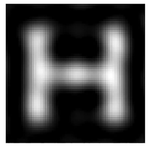
To motivate the use of HWT as a restriction operator, on the left of Figure 18, we can see the coarser version of $\mathbf{x}^{\mathrm{t}rue}$ defined by $\mathbf{x}^{(1)}=\mathbf{R}\mathbf{x}^{\mathrm{t}rue}$. This is a $32\times 32$ image that still conveys most of the information in the original $64\times 64$ image with the letter H, which demonstrates that reconstructing a coarse version may be enough for some applications. This can allow us to compress images to save storage space or bandwidth. For instance, suppose that before transmitting the image $\mathbf{b}$, we compute its coarser version $\mathbf{b}^{(1)}=\mathbf{R}\mathbf{b}$ and transmit just $\mathbf{b}^{(1)}$ (see right of Figure 18). The image $\mathbf{b}^{(1)}$ might have enough information to recover $\mathbf{x}^{(1)}$.

Figure 18.

The compressed true image $\mathbf{x}^{(1)}$ on the left and blurred and noisy image $\mathbf{b}^{(1)}$ on the right.

What is the right blurring matrix to recover $\mathbf{x}^{(1)}$ from $\mathbf{b}^{(1)}$? Using our example, we will show that using $\mathbf{A}^{(1)} = \mathbf{R}\mathbf{A}\mathbf{P}$ does a good job. Figure 19 shows the Tikhonov and TV solutions of the system $\mathbf{A}^{(1)}\mathbf{x}= \mathbf{b}^{(1)}$. Notice that we are solving a system with a $1,024 \times 1,024$ matrix instead of the original system with a $4,096\times 4,096$ matrix.

The following theorem shows that the HWT preserves the structures of the matrices described before.

Theorem 1 (7).

Let $\mathbf{T}$ be a $p\times p$ matrix with Toeplitz structure and with Toeplitz vector $\mathbf{t}$, and $p = 2^s$. Then, the $2^{s-1}\times 2^{s-1}$ matrix $\mathbf{T}^1 = \mathbf{W}_1\mathbf{T}\mathbf{W}^T_1$ is also Toeplitz with Toeplitz vector $\mathbf{t}_1 = \tilde{\mathbf{t}}(1: 2: 2p - 3)$, where $\tilde{\mathbf{t}}= \tilde{\mathbf{T}}\mathbf{t}$ with $\tilde{\mathbf{T}}$ being the Toeplitz matrix with Toeplitz vector with all zeros and $\mathbf{t}_0 = \mathbf{t}_{-2} = 1/2$ and $\mathbf{t}_{-1} = 1$.

Figure 19.

The reconstructed coarse images $\mathbf{x}^{\mathrm{reg}}$ of size $32\times 32$, obtained using the optimal regularization parameter and the discretization of the first derivative operator with the 2-norm regularization on the left, and TV regularization on the right.

A similar result can be shown for circulant matrices.

Corollary 1.

Let $\mathbf{C}$ be a $p\times p$ circulant matrix and $p = 2^s$. Then, the $2^{s-1} \times 2^{s-1}$ matrix $\mathbf{C}_1 = \mathbf{W}_1\mathbf{C}\mathbf{W}^T_1$ is also circulant.

Let us consider the case when $\mathbf{A}= \mathbf{A}_r \otimes \mathbf{A}_c \in \mathbb{R}^{m\times m}$. Then, by a property of the Kronecker product, we have that

$$\begin{align} \mathbf{A}^{(1)} &= (\mathbf{W}_1 \otimes \mathbf{W}_1) (\mathbf{A}_r \otimes \mathbf{A}_c) (\mathbf{W}_1 \otimes \mathbf{W}_1)^T \\ &= (\mathbf{W}_1\mathbf{A}_r\mathbf{W}^T_1)\otimes (\mathbf{W}_1\mathbf{A}_c\mathbf{W}^T_1)\\ &= \mathbf{A}^{(1)}_r\otimes \mathbf{A}^{(1)}_c. \end{align}$$

The matrix $\mathbf{A}^{(1)}\in \mathbb{R}^{(m/4)\times (m/4)}$ is separable. Furthermore, by Theorem 1, if $\mathbf{A}_r$ and $\mathbf{A}_c$ are Toeplitz matrices, then $\mathbf{A}^{(1)}_r$ and $\mathbf{A}^{(1)}_c$ are too. Applying this same argument repeatedly, we obtain that $\mathbf{A}^{(n)}$ is separable by two Toeplitz matrices and therefore BTTB for all levels $n = 0,\dots , L$. Similarly, by Corollary 1, $\mathbf{A}^{(n)}$ is separable by two circulant matrices and therefore BCCB for all levels $n = 0,\dots , L$. Therefore, the initial structure of the matrix is inherited by all the levels.

For the case when we have BCCB structures, we can solve the corresponding Tikhonov systems at all levels using Fourier-based methods. If we are dealing with separable matrices with Toeplitz structure, we could go down several levels until we can compute the SVD of $\mathbf{A}^{(n)}_r=\mathbf{U}^{(n)}_r\boldsymbol{\Sigma }^{(n)}_r(\mathbf{V}^{(n)}_r)^T$ and $\mathbf{A}^{(n)}_c=\mathbf{U}^{(n)}_c\boldsymbol{\Sigma }^{(n)}_c(\mathbf{V}^{(n)}_c)^T$, and use that

$$\begin{align} \mathbf{A}^{(n)} &= \mathbf{A}^{(n)}_r \otimes \mathbf{A}^{(n)}_c \\ &=(\mathbf{U}^{(n)}_r\boldsymbol{\Sigma }^{(n)}_r(\mathbf{V}^{(n)}_r)^T)\otimes (\mathbf{U}^{(n)}_c\boldsymbol{\Sigma }^{(n)}_c(\mathbf{V}^{(n)}_c)^T) \\ &=(\mathbf{U}^{(n)}_r\otimes \mathbf{U}^{(n)}_c)(\boldsymbol{\Sigma }^{(n)}_r\otimes \boldsymbol{\Sigma }^{(n)}_c)(\mathbf{V}^{(n)}_r\otimes \mathbf{V}^{(n)}_c)^T. \end{align}$$

This gives us basically the SVD of $\mathbf{A}^{(n)}$, except that the elements in the diagonal matrix $\boldsymbol{\Sigma }^{(n)}_r\otimes \boldsymbol{\Sigma }^{(n)}_c$ might not be in the decreasing order, and therefore some reordering would be needed.

10. Conclusions and Outlook

Our intention has been to introduce readers to the problem of image deblurring, the mathematical issues that arise, and a few techniques for addressing them. As mentioned in the introduction, these techniques may be applied to a wide range of related problems. Indeed, we outlined a number of alternative strategies, for example, in choosing appropriate boundary conditions or in selecting the best regularization parameter, as some strategies are better suited to a specific range of applications.

Most of the methods that we have described are primarily based around direct factorizations. However, when dealing with unstructured and very large matrices, iterative methods may need to be used instead. There is an extensive literature on iterative methods 18, but a discussion about them is outside the scope of this introductory article.

We believe this subject is accessible to both undergraduate and graduate students and can serve as a good introduction to inverse problems, working with ill-conditioned linear operators, and large-scale computation. The visual nature of the problem provides compelling motivation for students and allows the efficacy of various techniques to be easily assessed. Some introductory books on this subject include 111220.

In addition, this field is an active area of research that is connected to recent developments in machine learning and convolutional neural networks. For example, many classical techniques that have traditionally been used in image deblurring can be used to speed up the training of machine learning models, such as neural nets designed to classify images. Earlier we mentioned that Tikhonov regularization is related to ridge regression, a fundamental tool in machine learning. Indeed, the connection to machine learning goes much deeper.

The code to generate the figures appearing in this article is available at https://github.com/ipiasu/AMS_Notices_AEP. This manuscript contains only a limited number of references because journal rules restrict the maximum number of references to 20; additional references can also be found in the github link.