Euclidean Traveller in Hyperbolic Worlds

We will discuss all possible closures of a Euclidean line in various geometric spaces. Imagine the Euclidean traveller, who travels only along a Euclidean line. She will be traveling to many different geometric worlds, and our question will be what places does she get to see in each world?

Figure 1.

A Euclidean traveller.

Here is the itinerary of our Euclidean traveller:

•

In 1884, she travels to the torus of dimension $n\ge 2$, guided by Kronecker.

•

In 1936, she travels to the world, called a closed hyperbolic surface, guided by Hedlund Hed36.

•

In 1991, she then travels to a closed hyperbolic manifold of higher dimension $n\ge 3$ guided by Ratner Rat91.

•

Finally, she adventures into hyperbolic manifolds of infinite volume guided by Dal’bo Dal00 in dimension two in 2000, by McMullen-Mohammadi-O. MMO16 in dimension three in 2016 and by Lee-O. LO19 in all higher dimensions in 2019.

Rotations of the Circle

As a warm up, she will first do her exercise of jumping on the circle $\mathbb{S}^1$, which may be considered as the one-dimensional torus $\mathbb{T}^1$.

The circle $\mathbb{S}^1$ can be presented as

$$\mathbb{S}^1=\{z\in \mathbb{C}: |z|=1\} =\{z=e^{2\pi i x}:x\in \mathbb{R}\}.$$

In additive notation,

$$\mathbb{S}^1= \mathbb{Z}\backslash \mathbb{R}.$$

These two models are isomorphic to each other by the logarithm map $z=e^{2\pi i x}\mapsto x\;(\text{mod }1)$.

Let $\mathsf{R}_\theta$ denote the rotation of $\mathbb{S}^1$ by angle $2\pi \theta$.

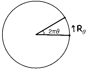
The map $\mathsf{R}_\theta$ is respectively given by

$$\mathsf{R}_\theta (z)= ze^{2\pi i \theta } \text{ and } \mathsf{R}_\theta (x)= x+\theta \quad \text{(mod $\mathbb{Z}$)}$$

in multiplicative and additive models of $\mathbb{S}^1$. The orbit of $z=e^{2\pi i x}\in \mathbb{S}^1$ under iterations of $\mathsf{R}_\theta$ is respectively equal to

$$\begin{equation*} \{ze^{2\pi i n \theta }: n\in \mathbb{Z}\}\text{ and } \{{{} x+n\theta } \;\; (\text{mod } 1): n\in \mathbb{Z}\}. \end{equation*}$$

Theorem 1.

Let $\theta \in \mathbb{R}$. Any orbit of $\mathsf{R}_\theta$ is closed or dense in $\mathbb{S}^1$, depending on whether $\theta$ is rational or not.

If our traveller keeps jumping by an irrational distance $\theta$, she is guaranteed to see all the places in the circle $\mathbb{Z}\backslash \mathbb{R}$.

Euclidean Lines on the Torus

$2$-torus

She travels to the $2$-torus $\mathbb{T}^2= \mathbb{Z}^2\backslash \mathbb{R}^2$. Let

$$\pi : \mathbb{R}^2\to \mathbb{T}^2= \mathbb{Z}^2\backslash \mathbb{R}^2$$

denote the canonical quotient map. A Euclidean line in $\mathbb{T}^2$ is the image of a line in $\mathbb{R}^2$ under $\pi$. For a nonzero vector $(\omega _1, \omega _2)\in \mathbb{R}^2$, we denote by

$$\begin{equation*} L_{\omega _1,\omega _2}=\pi (\mathbb{R}(\omega _1, \omega _2)) \end{equation*}$$

the image of the unique line passing through $(\omega _1, \omega _2)$ and the origin $(0,0)$. The slope of the line $\mathbb{R}(\omega _1, \omega _2)$ is equal to $\theta ={\omega _2}/{\omega _1}$.

What is the closure of the line $L_{\omega _1, \omega _2}$ in $\mathbb{T}^2$, or in other words, what places does our Euclidean traveller get to see in $\mathbb{T}^2$ if she travels along the line $L_{\omega _1, \omega _2}$?

Figure 2.

Torus.

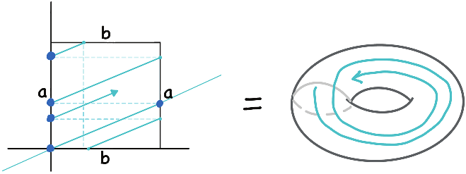
It is useful to consider the unit square $I^2=[0,1]\times [0,1]$ which is a fundamental domain of $\mathbb{Z}^2\backslash \mathbb{R}^2$. When we identify the pairs of opposite sides labelled by $a$ and $b$ in Figure 2 using the side pairing transformations $\gamma _a=(1,0)$ and $\gamma _b=(0,1)$ respectively, we get the torus $\mathbb{T}^2= \Gamma \backslash \mathbb{R}^2$ where $\Gamma =\mathbb{Z}^2$ is the subgroup generated by $\gamma _a$ and $\gamma _b$. The distribution of the line $L_{\omega _1, \omega _2}$ can be understood by examining the line $\mathbb{R}({\omega _1, \omega _2})$ inside $I^2$ modulo the action of $\mathbb{Z}^2$. In Figure 2, when our traveller, walking on the blue line $\mathbb{R}_{\omega _1, \omega _2}$ with slope $0<\theta <1$, reaches the boundary of $I^2$ at $(1, \theta )$, she gets instantly jumped to $(0, \theta )$ by the transformation $\gamma _a^{-1}=(-1,0)$, which also moves the line $\mathbb{R}(\omega _1, \omega _2)$ to the line with the same slope but passing through $(0, \theta )$. She then continues to walk on this new line in $I^2$ until she reaches the boundary of $I^2$. We can observe that the places on the circle $\{0\}\times [0,1)=\{0\}\times \mathbb{Z}\backslash \mathbb{R}$ that she is visiting are precisely given by the orbit $\{n\theta \; (\text{mod } 1 ): n\in \mathbb{N}\}$ of the rotation $\mathsf{R}_{\theta }$. Therefore by Theorem 1, if the slope $\theta =\omega _2/\omega _1$ is a rational number, she visits only finitely many points in $\{0\}\times \mathbb{Z}\backslash \mathbb{R}$, which means the line $L_{\omega _1, \omega _2}$ is periodic and hence closed in $\mathbb{T}^2$. Otherwise, the places she visits in $\{0\}\times \mathbb{Z}\backslash \mathbb{R}$ are dense, which means that the line is dense in $\mathbb{T}^2$.

Theorem 2 (Kronecker, 1884).

Any Euclidean line in $\mathbb{T}^2$ is closed or dense, depending on whether its slope is rational or not.

$n$-torus

For any $n\ge 2$, the $n$-torus $\mathbb{T}^n$ can be presented as $\mathbb{Z}^n\backslash \mathbb{R}^n$, and a line in $\mathbb{T}^n$ is the image of a line under the quotient map

$$\pi : \mathbb{R}^n\to \mathbb{T}^n=\mathbb{Z}^n\backslash \mathbb{R}^n.$$

For $(\omega _1, \cdots , \omega _n)\in \mathbb{R}^n$, let $L_{\omega _1, \cdots ,\omega _n}$ denote the line in $\mathbb{T}^n$ which is the image of the Euclidean line $\mathbb{R}(\omega _1, \cdots , \omega _n )$.

Figure 3.

Line in $\mathbb{T}^n$.

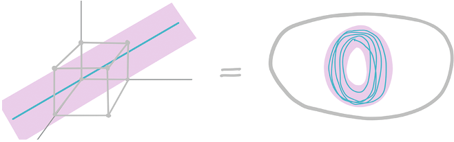
Unlike the dimension two case, the closed or dense dichotomy for a line is not true anymore in $\mathbb{T}^n$, $n\ge 3$, as $\mathbb{T}^n$ contains many lower dimensional tori. In Figure 3, the blue line $L$ is contained in a two-dimensional linear subspace $V<\mathbb{R}^3$ such that $\pi (V)$ is closed in $\mathbb{T}^2$ and $\overline{L}=\pi (V)=(V\cap \mathbb{Z}^3)\backslash V$. However, the lower dimensional tori are the only other possibilities (cf. KH95):

Theorem 3 (Kronecker).

For any nonzero $(\omega _1, \cdots , \omega _n)\in \mathbb{R}^n$, the closure of the line $L_{\omega _1, \cdots , \omega _n}$ is a $k$-dimensional subtorus of ${\mathbb{T}}^n$ where $k=\operatorname {dim}_{\mathbb{Q}} \sum _{i=1}^n \mathbb{Q} \omega _i$. That is, there exists a $k$-dimensional linear subspace $V<\mathbb{R}^n$ such that

$$\overline{L_{\omega _1, \cdots , \omega _n}}=\pi (V)=(V\cap \mathbb{Z}^n)\backslash V.$$

A general Euclidean torus is defined as the quotient

$$\Gamma \backslash \mathbb{R}^n$$

for some discrete cocompact subgroup $\Gamma$ of $\mathbb{R}^n$; a discrete subgroup $\Gamma$ of $\mathbb{R}^n$ is called cocompact if the quotient space $\Gamma \backslash \mathbb{R}^n$ is compact. It is not hard to prove that any discrete cocompact subgroup of $\mathbb{R}^n$ is of the form

$$\Gamma =\sum _{i=1}^n \mathbb{Z}v_i$$

for some basis $v_1$, …, $v_n$ of $\mathbb{R}^n$.

Theorem 4 (Kronecker).

For any line $L\subset \Gamma \backslash \mathbb{R}^n$ (not necessarily passing through the origin), there exists a linear subspace $V<\mathbb{R}^n$ such that

$$\overline{L}= (V\cap \Gamma )\backslash V \quad \text{up to translations}.$$

This seemingly more general theorem follows easily from Theorem 3 using the fact that $\overline{L +v}=\overline{L} +v$ for any $v\in \mathbb{Z}^n\backslash \mathbb{R}^n$ and $\Gamma = \mathbb{Z}^n g$ where $g$ is an element of $\operatorname {GL}_n(\mathbb{R})$ whose row vectors are given by $v_1$, …, $v_n$.

Closed Hyperbolic Surfaces

Our Euclidean traveller now wants to explore a world called a closed hyperbolic surface. A closed hyperbolic surface will be defined as a quotient of the hyperbolic plane $\mathbb{H}^2$.

Hyperbolic plane

The hyperbolic plane $\mathbb{H}^2$ is the unique simply connected two-dimensional complete Riemannian manifold of constant sectional curvature $-1$. Instead of this fancy description, we will be using a very explicit model, called the Poincaré upper half-plane model of $\mathbb{H}^2$. That is,

$$\mathbb{H}^2=\{(x,y)\in \mathbb{R}^2: y>0\}$$

with the hyperbolic metric given by $ds=\tfrac{\sqrt {dx^2+dy^2}}{y}$. This means that the hyperbolic distance between $p,q\in \mathbb{H}^2$ is defined as

$$d(p, q)=\inf \left\{\int _0^1 \tfrac{\|c'(t)\| }{y(t)} dt\right\}$$

where $c:[0,1]\to \mathbb{H}^2$, $c(t)=(x(t), y(t))$, ranges over all differentiable curves with $c(0)=p$ and $c(1)=q$. Because the hyperbolic distance is the Euclidean distance scaled by the Euclidean height of the $y$-coordinate, the hyperbolic distance between two points in $\mathbb{H}^2$ is larger (resp. smaller) than their Euclidean distance if their Euclidean height is small (resp. large).

Figure 4.

Upper half-plane model of $\mathbb{H}^2$.

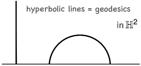
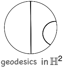
Geodesics, that is, distance-minimizing curves, in this upper half-plane model are half-lines or semicircles, perpendicular to the $x$-axis. In other words, to travel from a point $p$ to $q$ in the fastest way, one has to take the route given by the unique circle (or a line) passing through $p$ and $q$, perpendicular to the $x$-axis.

Another useful model is the Poincaré unit disk model in which $\mathbb{H}^2=\{x^2+y^2<1\}$ is the open unit disk in $\mathbb{R}^2$ and the hyperbolic metric is given by $ds=\tfrac{2\sqrt {dx^2+dy^2}}{1-(x^2+y^2)}$.

Geodesics in this model are lines or semicircles meeting the boundary $\mathbb{S}^1$ orthogonally.

Recall that

•

a Euclidean $2$-torus is given by a quotient$$\Gamma \backslash \mathbb{R}^2$$

where $\Gamma$ is a discrete cocompact subgroup of $\mathbb{R}^2$.

In analogy, we wish to be able to say that

•

a closed hyperbolic surface is given by a quotient$$\Gamma \backslash \mathbb{H}^2$$

where $\Gamma$ is a discrete cocompact subgroup of $\mathbb{H}^2$.

Alas, the hyperbolic plane $\mathbb{H}^2$ is not a group which makes this statement nonsense. However, $\mathbb{H}^2$ is “almost” the same as the group $\operatorname {Isom}^+(\mathbb{H}^2)$ of orientation preserving isometries of $\mathbb{H}^2$.

Isometry group of $\mathbb{H}^2$

On the upper half-plane model $\mathbb{H}^2=\{z=x+iy: y>0\}$, now considered as the set of complex numbers with positive imaginary parts, the group $\operatorname {PSL}_2(\mathbb{R})$ acts by linear fractional transformations:

$$\begin{pmatrix} a&b\\ c& d \end{pmatrix} z=\frac{az+b}{cz+d};$$

since $\operatorname {Im} \frac{az+b}{cz+d}=\frac{\operatorname {Im}(z)}{|cz+d|^2}$, this action preserves $\mathbb{H}^2$. We can also check that this action preserves the hyperbolic metric of $\mathbb{H}^2$. Therefore every element of $\operatorname {PSL}_2(\mathbb{R})$ is an isometry of $\mathbb{H}^2$. Moreover, it turns out that every orientation preserving isometry arises in this manner, yielding the identification

$$\operatorname {PSL_2}(\mathbb{R}) =\operatorname {Isom}^+(\mathbb{H}^2) .$$

It is easy to see that this action of $\operatorname {PSL_2(\mathbb{R})}$ on $\mathbb{H}^2$ is transitive with the stabilizer of $i$ being equal to the rotation group $\operatorname {SO}(2)$. Therefore the orbit map $\operatorname {PSL}_2(\mathbb{R})\to \mathbb{H}^2$, $g\mapsto g(i)$, induces the identification

$$\operatorname {PSL_2}(\mathbb{R})/\operatorname {SO}(2)=\mathbb{H}^2.$$

So modulo the compact subgroup $\operatorname {SO}(2)$, the hyperbolic plane $\mathbb{H}^2$ is equal to its isometry group $\operatorname {PSL}_2(\mathbb{R})$.

Closed hyperbolic surfaces

Definition 1.

A closed hyperbolic surface is a quotient

$$\Gamma \backslash \mathbb{H}^2$$

where $\Gamma$ is a discrete (torsion-free) cocompact subgroup of $\operatorname {PSL}_2(\mathbb{R})$.

By the quotient $\Gamma \backslash \mathbb{H}^2$, we mean the set of equivalence classes of elements of $z\in \mathbb{H}^2$ where $[z_1]=[z_2]$ if and only if $z_1=\gamma z_2$ for some $\gamma \in \Gamma$. The discreteness of $\Gamma$ implies that $\Gamma \backslash \mathbb{H}^2$ is locally $\mathbb{H}^2$ and the cocompactness of $\Gamma$ in $\operatorname {PSL}_2(\mathbb{R})$ implies that $\Gamma \backslash \mathbb{H}^2=\Gamma \backslash \operatorname {PSL}_2(\mathbb{R})/\operatorname {SO}(2)$ is compact.

Figure 5.

Hyperbolic octagon.

Does there exist a closed hyperbolic surface? Equivalently, does there exist a discrete cocompact subgroup of $\operatorname {PSL}_2(\mathbb{R})$? To present an example, consider the hyperbolic regular octagon $\mathsf{O}$ as illustrated in Figure 5, where each side is a hyperbolic geodesic segment of same length and angles between them are $45^\circ$.

For the two sides of the octagon labelled by $a$, there exists an isometry $\gamma _a\in \operatorname {PSL}_2(\mathbb{R})$ which moves one to the other. Similarly, we have $\gamma _b, \gamma _c,\gamma _d\in \operatorname {PSL}_2(\mathbb{R})$ for labels $b, c, d$ respectively. Let

$$\Gamma =\langle \gamma _a, \gamma _b, \gamma _c, \gamma _d\rangle <\operatorname {PSL}_2(\mathbb{R})$$

be the subgroup generated by these four side-pairing transformations. Then the hyperbolic octagon $\mathsf{O}$ is a fundamental domain for the action of $\Gamma$ in $\mathbb{H}^2$, which implies that $\Gamma$ is a discrete cocompact subgroup of $\operatorname {PSL}_2(\mathbb{R})$. The closed hyperbolic surface $\Gamma \backslash \mathbb{H}^2$ is what we obtain by gluing the four pairs of edges of the hyperbolic octagon according to labels; it is topologically a two-holed torus, or genus-two surface.

Any closed hyperbolic surface is topologically a closed surface with genus at least $2$. Conversely, the Uniformization theorem says that any closed surface with genus at least $2$ can be realized as a closed hyperbolic surface. Indeed, for any $g\ge 2$, the space of all marked closed hyperbolic surfaces of genus is homeomorphic to $\mathbb{R}^{6g-6}$.

Figure 6.

Surface with genus $g\ge 2$.

Now that our traveller learned that there exist many (even a continuous family of) closed hyperbolic surfaces to explore, she has to understand what a Euclidean line is in this world.

Euclidean Lines in Closed Hyperbolic Surfaces

In the upper half-plane model of $\mathbb{H}^2$, the horizontal line $\{y=1\}$ will be called a Euclidean line in $\mathbb{H}^2$. In a given geometric space, objects which are isometric to each other should be given the same name. We note that the image of $\{y=1\}$ under an isometry of $\mathbb{H}^2$ is either another horizontal line, or a circle which is tangent to the $x$-axis. So all of these objects will be called Euclidean lines in $\mathbb{H}^2$. A nickname for a Euclidean line is a horocycle. A horocycle in $\mathbb{H}^2$ is characterized as an isometric embedding of the real line $\mathbb{R}$ to $\mathbb{H}^2$ with constant curvature one; geodesics in $\mathbb{H}^2$ have constant curvature zero.

Figure 7.

Euclidean lines in $\mathbb{H}^2$.

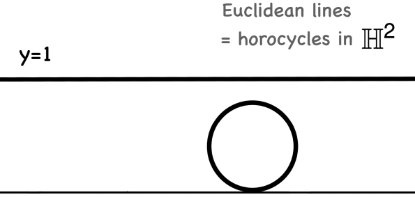
From the point of view of our Euclidean traveller, imagine that she wants to drive in a car where the steering wheel is in one fixed position and to travel without bumps. If her car is turning at a constant rate, she can lean back against the seat, feeling stable. It’s the change in curvature that makes the car trip bumpy. If the wheel is fixed at a small angle, she stays within a bounded distance of a geodesic. If the wheel is fixed at a large angle, she goes around in a circle and stays a bounded distance from a point. But in between there is a perfect angle where neither happens, and she moves along a horocycle!

A Euclidean line in a closed hyperbolic surface $\Gamma \backslash \mathbb{H}^2$ is the image of a Euclidean line in $\mathbb{H}^2$ under the quotient map

$$\pi : \mathbb{H}^2\to \Gamma \backslash \mathbb{H}^2.$$

Where does our Euclidean traveller get to visit in a closed hyperbolic surface?

Figure 8.

Traveling along a Euclidean line.

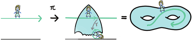
Here is an illustration given in Figure 8. Fix a (blue-colored) fundamental domain $\mathsf{O}$ for $\Gamma \backslash \mathbb{H}^2$. When the traveller, walking along the mint-colored Euclidean line $L$, reaches the boundary of $\mathsf{O}$, she gets instantly moved to a different side of $\mathsf{O}$ by some side-pairing transformation $\gamma \in \Gamma$. She then continues her journey on the new Euclidean line $\gamma (L)$ inside $\mathsf{O}$ until she reaches the boundary of $\mathsf{O}$ again, etc. The instant jumps and the shapes of translates of $L$ made by $\Gamma$ in $\mathbb{H}^2$ appear more complicated than those in the Euclidean torus $\mathbb{T}^2$.

Nevertheless, Hedlund (1936) assures that our Euclidean traveller gets to see all the places in a closed hyperbolic surface, no matter where her initial point of departure is.

Theorem 5.

Hed36 Any Euclidean line in a closed hyperbolic surface is dense.

Figure 9.

Euclidean traveller.

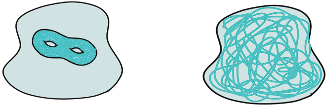
Hyperbolic lines can be very wild

We remark that this theorem of Hedlund is about Euclidean lines. The closure of a hyperbolic line does not even have to be a submanifold in general.

Figure 10.

Hyperbolic traveller.

As illustrated in Figure 10, a geodesic can “spiral” around closed geodesics and its closure can be a fractal of dimension strictly between one and two.

Going upstairs

Hedlund’s proof of Theorem 5 relies on the fact that $\mathbb{H}^2$ is almost $\operatorname {PSL}_2(\mathbb{R})$. The isometric action of $\operatorname {PSL}_2(\mathbb{R})$ on $\mathbb{H}^2$, which gave us the identification $\mathbb{H}^2=\operatorname {PSL}_2(\mathbb{R})/\operatorname {SO}(2)$, extends to an action on the unit tangent bundle $\operatorname {T}^1(\mathbb{H}^2)$. In this action, the stabilizer of a vector is trivial, as no rotation in the plane fixes a vector. If we denote $v_0\in \operatorname {T}^1(\mathbb{H}^2)$ the upward normal vector based at $i$, then the orbit map $g\mapsto g(v_0)$ now gives an isomorphism $\operatorname {PSL}_2(\mathbb{R})=\operatorname {T}^1(\mathbb{H}^2)$, where the identity matrix of $\operatorname {PSL}_2(\mathbb{R})$ corresponds to the vector $v_0$. Moreover, if we consider the following one-dimensional subgroup

$$U=\left\{\begin{pmatrix} 1& t \\ 0 &1\end{pmatrix}: t\in \mathbb{R}\right\},$$

then the subgroup $U$ corresponds to the set of all upward normal vectors on the Euclidean line $\{y=1\}$ (see Figure 11).

Figure 11.

$U$-orbits.

Similarly, for $g\in \operatorname {PSL}_2(\mathbb{R})$ with $g\{y=1\}$ a circle tangent at $\xi$, the coset $gU$ corresponds to the set of all inward normal vectors on $g\{y=1\}$ pointing to $\xi$. Indeed, any Euclidean line (EL) in $\mathbb{H}^2$ arises as the image of some $gU$ under the basepoint projection map $\operatorname {PSL}_2(\mathbb{R})=\operatorname {T}^1(\mathbb{H}^2)\to \mathbb{H}^2$ given by $g\mapsto g(i)$:

$$\begin{equation*} \boxed { \begin{array}{ccccc} \operatorname {T}^1( \mathbb{H}^2) & = & \operatorname {PSL}_2(\mathbb{R}) & \supset gU \\& \downarrow & & \downarrow \\\mathbb{H}^2 &=& \operatorname {PSL}_2(\mathbb{R})/\operatorname {SO}(2) & \supset \text{EL} \\\end{array} } \end{equation*}$$

Since the image of $gU$ in $\Gamma \backslash \operatorname {PSL}_2(\mathbb{R})$, under the projection $\operatorname {PSL}_2(\mathbb{R})\to \Gamma \backslash \operatorname {PSL}_2(\mathbb{R})$, is equal to $\Gamma \backslash \Gamma gU$ and $\mathbb{H}^2=\operatorname {PSL}_2(\mathbb{R})/\operatorname {SO}(2)$, this picture is preserved under the quotient map $\pi :\mathbb{H}^2\to \Gamma \backslash \mathbb{H}^2$:

$$\begin{equation*} \boxed { \begin{array}{cccc} \operatorname {T}^1(\Gamma \backslash \mathbb{H}^2) & = & \Gamma \backslash \operatorname {PSL}_2(\mathbb{R}) & \supset xU \\& \downarrow & & \downarrow \\\Gamma \backslash \mathbb{H}^2 &=& \Gamma \backslash \operatorname {PSL}_2(\mathbb{R})/\operatorname {SO}(2) & \supset \text{EL} \\\end{array} } \end{equation*}$$

It follows that any Euclidean line in $\Gamma \backslash \mathbb{H}^2$ is of the form $xU (i)$ and $\overline{xU(i)}= \overline{xU} (i)$, as the basepoint projection map $g\to g(i)$ has compact fibers. Therefore if we can describe the closures of all orbits $xU$ in $\Gamma \backslash G$, we understand the closure of a Euclidean line in $\Gamma \backslash \mathbb{H}^2$.

Figure 12.

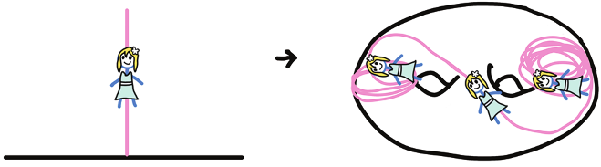
Traveling with an arrow.

Indeed, Hedlund says that every $U$-orbit is dense upstairs in $\operatorname {T}^1(\Gamma \backslash \mathbb{H}^2)$:

Theorem 6.

Hed36 For any $x\in \Gamma \backslash \operatorname {PSL}_2(\mathbb{R})$,

$$\overline{xU}=\Gamma \backslash \operatorname {PSL}_2(\mathbb{R}).$$

This means that our Euclidean traveller in a closed hyperbolic surface not only gets to see all the places, but she is able to appreciate those places from all angles as in Figure 9.

Closed Hyperbolic $n$-manifolds

For $n\ge 2$, the hyperbolic $n$-space $\mathbb{H}^n$ is the unique simply connected complete $n$-dimensional Riemannian manifold of constant sectional curvature $-1$. Its upper half space model is given by

$$\mathbb{H}^n=\{(x_1, \cdots , x_{n-1},y): y>0\}$$

with the hyperbolic metric $ds=\tfrac{\sqrt {dx_1^2+\cdots +dx_{n-1}^2+dy^2}}{y}$. In this model, geodesics are vertical lines or semicircles meeting the hyperplane $\mathbb{R}^{n-1}\times \{0\}$ orthogonally.

The hyperboloid model (also called the Minkowski model) of $\mathbb{H}^n$ is given by $\{Q_0(x_1, \cdots , x_{n+1})=-1, x_{n+1}>0\}$ where

$$\begin{equation} Q_0(x_1, \cdots , x_{n+1})=x_1^2 +x_2^2+\cdots + x_n^2 -x_{n+1}^2 .{\tag{1}} \end{equation}$$

In this model, the hyperbolic distance $d(x, y)$ is given by $\cosh d(x,y)= -Q_0(x,y)$ (cf. Rat94). In particular, any element $g$ of the special orthogonal group $\operatorname {SO}(Q_0)$, that is, $g\in \operatorname {SL}_{n+1}(\mathbb{R})$ satisfying

$$Q_0(g v)= Q_0(v)\text{ for all $v\in \mathbb{R}^{n+1}$},$$

is an isometry of $\mathbb{H}^n$. Indeed, the group $\operatorname {Isom}^+(\mathbb{H}^n)$ of orientation preserving isometries is given by the identity component of the special orthogonal group $\operatorname {SO}(Q_0)$; so

$$\operatorname {Isom}^+(\mathbb{H}^n)\simeq \operatorname {SO}^\circ (n,1).$$

This is consistent with our previous statement that $\operatorname {Isom}^+(\mathbb{H}^2)=\operatorname {PSL}_2(\mathbb{R})$, since $\operatorname {PSL_2}(\mathbb{R})\simeq \operatorname {SO}^\circ (2,1)$. As in the dimension two case, we have

•

any closed hyperbolic $n$-dimensional manifold is a quotient$$M=\Gamma \backslash \mathbb{H}^n$$

where $\Gamma$ is a discrete (torsion-free) cocompact subgroup of $\operatorname {SO}^\circ (n,1)$.

Unlike the dimension two case where there is a continuous family of closed hyperbolic surfaces, higher dimensional closed hyperbolic manifolds are rarer. The Mostow rigidity theorem Mos73 implies that there exist only countably many closed hyperbolic manifolds of dimension at least three. Nevertheless, there are infinitely many of them Bor63.

In the upper half-space model $\mathbb{H}^n=\{(x_1, \cdots , x_{n-1},y): y>0\}$, the horizontal line $\{(x_1, 0, \cdots , 0, 1): x_1\in \mathbb{R}\}$, and its isometric images will be called a Euclidean line (=horocycle) in $\mathbb{H}^n$. As before, a Euclidean line in $M=\Gamma \backslash \mathbb{H}^n$ is the image of an Euclidean line in $\mathbb{H}^n$ under the canonical quotient map $\pi : \mathbb{H}^n\to \Gamma \backslash \mathbb{H}^n$. They are isometric immersions of $\mathbb{R}$ with zero torsion and constant curvature $1$. What places does our Euclidean traveller get to see in $M$?

Figure 13.

Euclidean traveller in $\Gamma \backslash \mathbb{H}^n$.

The answer to this question is a special case of Ratner’s theorem on orbit closure classification.

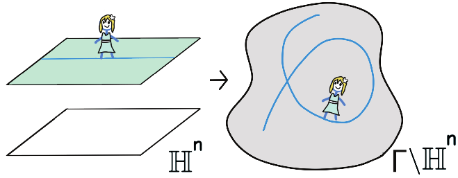
Homogeneous Dynamics

Let $G$ be a connected simple linear Lie group. (e.g., $\operatorname {SL}_n(\mathbb{R}), \operatorname {SO}^\circ (n,1)$), and $\Gamma <G$ be a discrete subgroup. The quotient space $\Gamma \backslash G$ is a homogeneous space, in the sense that there is a transitive action of a Lie group, which is $G$ in our case. Any subgroup $U$ of $G$ acts on this homogeneous space $\Gamma \backslash G$ by translations on the right, giving rise to a topological dynamical system:

$$\Gamma \backslash G \curvearrowleft U.$$

Studying dynamical properties of subgroup action on a homogeneous space $\Gamma \backslash G$ is a main subject in the field of homogeneous dynamics. A fundamental question in homogeneous dynamics is whether one can understand all possible orbit closures:

Question 2.

For a given point $x\in \Gamma \backslash G$, what is the closure $\overline{xU}?$

Moore’s ergodicity theorem Moo66 implies that if the homogeneous space $\Gamma \backslash G$ is compact, or more generally is of finite volume, then for any non-compact subgroup $U$ of $G$, almost all $U$-orbits are dense, that is, for almost all $x\in \Gamma \backslash G$,

$$\overline{xU}=\Gamma \backslash G .$$

Indeed, a hyperbolic line in a closed hyperbolic surface $\Gamma \backslash \mathbb{H}^2$ is the image of an orbit of the diagonal subgroup $A=\{{\begin{pmatrix} e^{t} & 0\\ 0&e^{-t}\end{pmatrix}}:t\in \mathbb{R}\}$ of $\operatorname {PSL}_2(\mathbb{R})$ under the basepoint projection $\Gamma \backslash \operatorname {PSL}_2(\mathbb{R})=\operatorname {T}^1(\Gamma \backslash \mathbb{H}^2)\to \Gamma \backslash \mathbb{H}^2$; hence this theorem implies that almost all hyperbolic lines are dense in a closed hyperbolic surface.

The weakness of this ergodicity theorem is that it is only the existence of many dense orbits. If one specifies the initial point $x$, it gives no information about the closure of the given orbit $xU$.

The following celebrated theorem of Ratner fixes this weakness for unipotent subgroup actions, answering the conjecture of Raghunathan in the affirmative.

A matrix $u$ is called unipotent if all of its eigenvalues are equal to $1$. For instance, $u_t=\begin{pmatrix} 1& t \\ 0 &1\end{pmatrix}$ is unipotent but $a_t=\begin{pmatrix} e^{t} & 0\\ 0&e^{-t}\end{pmatrix}$ is not unipotent for $t\ne 0$.

Theorem 7.

Rat91 Let $\operatorname {Vol}(\Gamma \backslash G)<\infty$ and $U$ be a connected subgroup of $G$ generated by unipotent elements. For any $x\in \Gamma \backslash G$,

$$\overline{xU}=xH$$

for some closed connected subgroup $H$ of $G$ which contains $U$.

Back to Euclidean Lines in Closed Hyperbolic Manifolds

Given a closed hyperbolic manifold $M=\Gamma \backslash \mathbb{H}^n$, its frame bundle $\operatorname {F}(M)$, consisting of positively oriented orthonomal frames on $M$, is identified with the homogeneous space $\Gamma \backslash \operatorname {SO}^\circ (n,1)$, as the action of $\operatorname {Isom}^+(\mathbb{H}^n)=\operatorname {SO}^\circ (n,1)$ is simply transitive on $\operatorname {F}(\mathbb{H}^n)$. Moreover, we have a one-dimensional subgroup $U$ of $\operatorname {SO}^\circ (n,1)$ given by

$$U=\left\{\begin{pmatrix} 1& t & 0 & \cdots & 0 & -t^2/2\\ 0 & 1 & 0 &\cdots & 0 & -t\\ 0 & 0 & 1 &\cdots & 0 & 0 \\ \vdots & \vdots & \vdots & \vdots & \vdots & \vdots \\ 0 &0 &0 &0 &1 & 0\\ 0 &0 &0 &0 &0 & 1\end{pmatrix} :t\in \mathbb{R}\right\}$$

(up to conjugation) such that every Euclidean line (EL) in $M$ is the image of some $U$-orbit in $\Gamma \backslash \operatorname {SO}^\circ (n,1)$ under the basepoint projection map:

$$\begin{equation*} \boxed { \begin{array}{ccccc} \operatorname {F}(\Gamma \backslash \mathbb{H}^n) & = & \Gamma \backslash \operatorname {SO}^\circ (n,1) & \supset xU \\& \downarrow & & \downarrow \\& \Gamma \backslash \mathbb{H}^n& & \supset \text{EL} \\\end{array} } \end{equation*}$$

Since $U$ consists of unipotent elements, Ratner’s theorem 7 applies to orbits of $U$.

For each integer $1\le k\le n$, we set $\mathcal{H}_k \coloneq \{(x_1, \cdots , x_{k-1}, 0, \cdots , 0, y)\in \mathbb{H}^n\}$. A hyperbolic $k$-subspace of $\mathbb{H}^n$, which will be denoted by $\mathbb{H}^k$, is an isometric image of $\mathcal{H}_k$, that is, $g (\mathcal{H}_k)$ for some $g\in \operatorname {Isom}^+(\mathbb{H}^n)$.

Definition 3.

By a closed hyperbolic (properly immersed) $k$-submanifold of $M$, we mean the compact image

$$\pi (\mathbb{H}^k)\subset \Gamma \backslash \mathbb{H}^n$$

for a hyperbolic $k$-subspace $\mathbb{H}^k\subset \mathbb{H}^n$.

Note that for any $k\ge 2$, a closed hyperbolic $k$-submanifold of $M$ contains many dense Euclidean lines. So certainly, if $M$ possesses a closed hyperbolic $k$-submanifold $N$, then some Euclidean lines lying in $N$ will have their closures equal to $N$. There are other possibilities for the closure of a Euclidean line in $M$. To explain what they are, we introduce the notion of a tilting of a hyperbolic subspace, which is analogous to a translation of a subspace by a vector in the Euclidean space $\mathbb{R}^n$.

Figure 14.

Tilted hyperbolic subspace.

Definition 4 (Tilting).

For a given hyperbolic $k$-subspace $\mathbb{H}^k$ of $\mathbb{H}^n$ for $1\le k\le n-1$, choose a hyperbolic subspace $\mathbb{H}^{k+1}$ containing $\mathbb{H}^k$ equipped with an orientation, and a nonnegative number $d_0\ge 0$. For $x\in \mathbb{H}^{k}$, let $\mathsf{T} (x)\in \mathbb{H}^{k+1}$ be the unique point lying in the geodesic determined by the outward normal vector to $\mathbb{H}^{k}$ and $d(x,\mathsf{T} (x))=d_0$. We call $\mathsf{T}:\mathbb{H}^k\to \mathbb{H}^{k+1}$ a tilt map and its image $\mathsf{T}(\mathbb{H}^{k})$ a tilted hyperbolic $k$-subspace of $\mathbb{H}^n$ (Figure 14).

The significance of a tilt map relevant to our discussion is that the image of a Euclidean line lying in $\mathbb{H}^k$ under a tilt map is a Euclidean line and that if $N=\pi (\mathbb{H}^k)$ is a closed hyperbolic submanifold of $M$, then $\pi (\mathsf{ T}(\mathbb{H}^k))$ is also a compact submanifold which is equidistant from $\pi (\mathbb{H}^k)$. Noting that a tilt map commutes with isometric action of $G$, the following

$$\mathsf{ T} (N)= \pi (\mathsf{ T}(\mathbb{H}^k))$$

is well-defined; we call $\mathsf{ T} (N)$ a tilting of a hyperbolic manifold $N$. If a Euclidean line $L$ is dense in $N=\pi (\mathbb{H}^k)$, then $\mathsf{ T}(L)$ is dense in $\mathsf{ T} (N)$.

Now the following consequence of Ratner’s theorem Rat91 implies that these are all possible closures of a Euclidean line.

Figure 15.

Closures of Euclidean lines.

Theorem 5.

Let $M=\Gamma \backslash \mathbb{H}^n$ be a closed hyperbolic $n$-manifold for $n\ge 2$. Then the closure of any Euclidean line in $M$ is a closed hyperbolic submanifold, up to tilting.

Therefore, no matter where she starts her journey, our Euclidean traveller in a closed hyperbolic world is guaranteed to see all the places of some hyperbolic subworld or at least a tilted version of it.

Traveling only in one direction

From a traveller’s point of view, a natural question to the travel guide is whether she can still sightsee the same places by walking only in one direction, in other words, is the closure of a half Euclidean line in a closed hyperbolic manifold the same as the closure of the whole Euclidean line? The answer is yes by the following version of Ratner’s theorem:

Theorem 8.

Rat91 Let $\operatorname {Vol}{(\Gamma \backslash G)}<\infty$ as in Theorem 7, and let $U=\{u_t:t\in \mathbb{R}\}$ be a one-parameter subgroup of unipotent elements. For any $x\in \Gamma \backslash G$,

$$\begin{equation} \overline{xU}=\overline{xU^{+}} {\tag{2}} \end{equation}$$

where $U^{+}=\{u_{t}: t\ge 0\}$.

Hyperbolic Manifolds of Infinite Volume

After adventuring all closed hyperbolic manifolds, our Euclidean traveller is now ready to venture into a hyperbolic manifold of infinite volume. Will she again be able to see all the places of some hyperbolic subworld?

It turns out that there are certain hyperbolic manifolds homeomorphic to the product of a closed surface and $\mathbb{R}$ where some Euclidean lines have wild closures. On the other hand, our wonderful travel agency presents a list of infinitely many hyperbolic manifolds of infinite volume where similar well-planned sightseeing is possible as in closed hyperbolic manifolds. This class of hyperbolic manifolds are called hyperbolic manifolds with Fuchsian ends. They are all obtained from closed hyperbolic manifolds by a certain removing and growing process; we may think of them as children of closed hyperbolic manifolds.

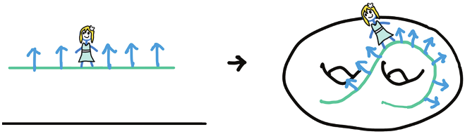
Hyperbolic Surfaces with Fuchsian Ends

We first explain how to construct a hyperbolic surface with Fuchsian ends as illustrated in Figure 16. For any closed hyperbolic surface $S=\Gamma _0\backslash \mathbb{H}^2$, choose a simple closed geodesic $\mathcal{L}$ ($S$ contains infinitely many such), which may or may not be separating.

Figure 16.

Hyperbolic surface with Fuchsian ends.

After removing $\mathcal{L}$ from $S$, we get a hyperbolic surface $N_0$ whose boundary is one or two copies of $\mathcal{L}$, depending on whether $\cal L$ is separating or not. If we let each boundary component grow naturally in hyperbolic world, we get a hyperbolic surface with Fuchsian ends. In other words, there is a canonical way to extend $N_0$ to a complete hyperbolic surface which is homeomorphic to $N_0$, namely, by gluing the continuous stack $\mathcal{L}\times [0,\infty )=\{\mathcal{L}^t: t\in [0, \infty )\}$ of titled hyperbolic lines to each boundary component of $N_0$. The resulting hyperbolic surface is of the form $N=\Gamma \backslash \mathbb{H}^2$ where $\Gamma <\Gamma _0$ is the fundamental group of $N_0$. This is an example of a hyperbolic surface with Fuchsian ends (Figure 16).

More generally, a hyperbolic surface with Fuchsian ends is obtained from a closed hyperbolic surface $S$ by a similar procedure for a finite set of disjoint simple closed geodesics $\{\mathcal{L}_1, \cdots , \mathcal{L}_k\}$. A connected surface, say $N_0$, of $S-\bigcup _i \mathcal{L}_i$ is a hyperbolic surface with boundary components and the resulting complete hyperbolic surface, say, $N$, obtained by gluing the corresponding hyperbolic cylinders to each boundary component is a hyperbolic surface with Fuchsian ends. The metric closure of $N_0$ is a compact hyperbolic surface which is homotopy-equivalent to $N$. By a hyperbolic surface with Fuchsian ends, we mean a surface obtained in this way.

In any hyperbolic surface with (non-empty) Fuchsian ends, there exist many Euclidean lines contained in the end of $N$, that is, in $N-N_0$, and they, as well as Euclidean lines which are equidistant from them, are proper immersions of the Euclidean line in $\mathbb{H}^2$ via $\pi$.

The following theorem of Dal’bo, which extends Hedlund’s theorem 5, says that they are the only possible non-dense Euclidean lines.

Theorem 9.

Dal00 If $N$ is a hyperbolic surface with Fuchsian ends, any Euclidean line in $N$ is closed or dense.

So our Euclidean traveller will simply disappear from the hyperbolic world or she will be seeing all the places even including the Fuchsian ends. There is a friendly warning in the pamphlet that walking along a half line won’t take her to all the places she would be seeing on the full line unlike closed hyperbolic manifolds.

Hyperbolic $n$-manifolds with Fuchsian Ends

Figure 17.

Hyperbolic manifold with one Fuchsian end.

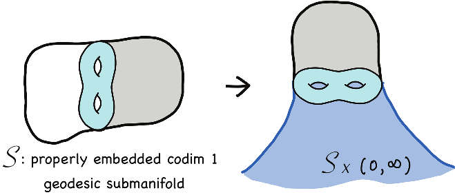
A hyperbolic $n$-manifold with Fuchsian ends for $n\ge 3$ is constructed similarly to the surface case, based on the observation that simple closed geodesics describe all properly embedded hyperbolic submanifolds of a closed hyperbolic surface of codimension one.

Recall that there are only countably many closed hyperbolic $n$-manifolds for $n\ge 3$. There are infinitely many of them (though not all) which contain properly embedded hyperbolic submanifolds of codimension one. Take one such closed hyperbolic $n$-manifold $M$ with a properly embedded hyperbolic submanifold $\mathcal{S}$ of codimension one; see the illustration in Figure 17.

A connected component $N_0$ of $M-\mathcal{S}$ is a hyperbolic manifold with one or two totally geodesic boundary components isometric to $S$. If we let $N_0$ naturally grow in the hyperbolic world, or if we glue the continuous stack $\mathcal{S}\times [0, \infty )=\{\mathcal{S}^t: t\in [0, \infty )\}$ of tilted hyperbolic submanifolds to each boundary component of $N_0$, we obtain a complete hyperbolic $n$-manifold $N$, homeomorphic to its submanifold $N_0$. This is a hyperbolic manifold with Fuchsian ends; connected components of $N-N_0$ are called Fuchsian ends of $N$.

Figure 18.

Hyperbolic manifold with 3 Fuchsian ends.

As in the surface case, we mean by a hyperbolic manifold with Fuchsian ends a complete hyperbolic manifold obtained from a closed hyperbolic manifold with a choice of finitely many disjoint properly embedded hyperbolic submanifolds of codimension one.

We may regard a closed hyperbolic manifold as a hyperbolic manifold with empty Fuchsian ends.

Theorem 10 (MMO17, MMO16 for $n=3$, and LO19 for all $n\ge 4$).

Let $N=\Gamma \backslash \mathbb{H}^n$ be a hyperbolic manifold with Fuchsian ends for $n\ge 2$. Any Euclidean line in $N$ is closed or its closure is a hyperbolic submanifold with Fuchsian ends, up to tilting.

So our Euclidean traveller in a hyperbolic manifold with Fuchsian ends again finds herself either disappearing from the hyperbolic world or enjoys her sightseeing in some hyperbolic submanifold with Fuchsian ends, or at least a tilted version of it.