PDFLINK |
Steklov Spectrum and Elliptic Problems with Nonlinear Boundary Conditions
Communicated by Notices Associate Editor Daniela De Silva
Problems with nonlinear boundary conditions arise naturally in many applications. For instance, in population dynamics where an impact of habitat-edges (boundary) on the dispersal pattern of species as they reach the boundary takes place in spatial ecology CC06. They occur when the biochemical reactions take place at or near the boundary, for example, in the limb bud development of a chick in which a chemical reaction produces outgrowth due to cell growth and division, and interactions between morphogens produced in several zones of the limb bud DO99. They also appear in noninvasive testing methods to locate defects in a medium by using boundary data measurements (see, e.g., CCMM16). In cryosurgery (a minimally invasive treatment used to treat some types of cancers and some conditions that may become cancer), a highly exothermic reaction takes place in a thin layer around the boundary in order to destroy abnormal tissue LOS98. These examples are not exhaustive.
Diffusion-type equations play a crucial role in these problems, and associated steady state problem and eigenvalue problems are critical in understanding the dynamics of diffusion-type equations. Hence, the qualitative (analytical) study of such equations is essential for better understanding and modeling nonlinear processes. The investigation of problems with nonlinear boundary conditions has therefore attracted a lot of attention in recent years; see for instance Ama76MN10Mav12MP17LS18CL15 and references therein.
In this article, we first introduce the spectral problem for elliptic equations with spectral-parameter dependent boundary conditions. We then discuss some recent results on the solvability of nonlinear diffusion problems when the nonlinearity on the boundary interacts in some sense with the spectrum, especially the effect of the first eigenvalue. We will present some of the results without proofs. References will be mentioned as appropriate.
In the following sections, we will first consider the linear Steklov problem in which the spectral parameter is in the boundary condition. Then, we discuss in-depth the properties of the first eigenvalue as well as briefly consider the one-dimensional case. In the last section, we take up the case of nonlinear perturbations of the linear Steklov problem, and set up the problem as a nonlinear first-order boundary-flux equation with a second-order elliptic partial differential equation “constraint” inside the domain. Considering asymptotic conditions on the boundary nonlinearity, we present existence, bifurcation and multiplicity results. A sketch of the bifurcation diagram is also provided.
Steklov Spectrum and its Properties
In the seminal paper entitled “Sur les problèmes fondamentaux de la physique mathématique (suite et fin),” published in 1902 in the Annales Scientifiques de l’École Normale Supérieure Ste02, W. Steklov considered the (spectral) problem of finding a harmonic function inside a convex bounded region in the plane with smooth boundary surface which satisfies the boundary condition
where denotes the directional derivative in the direction of the (unit) outward normal vector to the boundary , is a spectral parameter, and is a given smooth positive (weight) function. The convexity condition on the region and the smoothness of the surface were relaxed by H. Poincaré, and the positive weight function was introduced by E. Le Roy. Soon after that S. Zaremba considered the more general (spectral) problem with a lower-order term
where is the Laplace operator and is a (fixed) constant.
Later on in Pay67, Payne presented a physical problem that describes the vibration of an elastic membrane with its whole mass uniformly distributed on the boundary with density leading to the problem
where denotes an -dimensional body with boundary .
There have been many results and generalizations of the Steklov problem. We mention the book by Bandle Ban80 and the papers by Auchmuty Auc04 and Mavinga Mav12 for higher dimensions with mild regularity conditions on the data. We refer also to Amann Ama76 who discussed the existence of the first eigenvalue of the spectrum for this problem under somewhat strong regularity conditions on the data. Although a more general linear operator with lower order terms was considered in Ama76, the techniques there used the theory of positive operators (Krein–Rutman theorem); which of course does not apply when trying to obtain higher eigenvalues. The arguments in Auc04, which yielded higher eigenvalues as well, involved maximization of the boundary functional on bounded closed convex subsets of the Sobolev space .
In this article, we present an approach used in Mav12 where the minimization of the (differential) functional on an appropriate subspace of is used.
Steklov eigenproblem
Let , , be a bounded domain with smooth boundary . Consider the second-order elliptic equation
where the (given) functions and the weight satisfy the following conditions.
- (C)
and are nonnegative functions such that and . Here, denotes the real Lebesgue space of bounded functions.
Throughout this article, denotes the usual real Sobolev space of functions on ; which is a Hilbert space endowed with the -inner product defined by
with the associated norm denoted by . This norm is equivalent to the standard -norm.
Besides the Sobolev spaces, we make use, in what follows, of the real Lebesgue space of square integrable functions, and the compactness of the trace operator (see, e.g., Bre11 and references therein). Sometimes we will just use in place of when considering the trace of a function on . We will denote the -inner product by and the associated norm by . We also set
for . Observe that because of condition (C), it can happen that in a subset of positive measure (on the boundary ) where . In this case is only a semi-norm. Set . It is readily seen that is a closed linear subspace of . Observe that if on , then the subspace reduces simply to . Let us denote the -orthogonal complement of by . Therefore, one can split
as a direct orthogonal sum (in the sense of --inner product); that is, every can be written in a unique way in the form , where and with .
The Steklov eigenproblem (in its variational form) is to find a pair with such that
for every . The real number is called an eigenvalue of 2 and the function is said to be an eigenfunction associated to the eigenvalue .
Now, choosing , one sees immediately that if there is such an eigenpair, then and . Otherwise, would be a constant function; which would contradict the assumption (C) imposed on . Therefore in the --inner product defined in 3 above. Notice also that, if with , then and the quotient .
The set of such that 2 has a nontrivial solution, is called the Steklov spectrum.
In what follows, we present some results on the properties of the Steklov spectrum. Namely that forms a countably infinite set without finite accumulation point. Thus, its elements can be arranged in an increasing sequence. We omit the details and refer to Mav12 for the proof.
Variational characterization of the Steklov spectrum
Assume that the condition (C) holds, then
- (i)
The Steklov eigenproblem 2 has a sequence of real eigenvalues
and these eigenvalues satisfy the variational characterizations
and for
where and are the eigenfunctions corresponding to . (Hence, each eigenvalue has a finite-dimensional eigenspace.)
- (ii)
The normalized eigenfunctions provide a complete -orthonormal basis of . Moreover, each function has a unique representation of the form
In addition
Observe that the variational characterization 6 gives the trace inequality
for all . Moreover if equality holds in 8, then is a multiple of an eigenfunction of Eq. 2 corresponding to .
On the other hand, for every and we have that
where denotes the -eigenspace and is the span of eigenfunctions associated to eigenvalues up to .
Hence, this gives a splitting of the space (and hence of ).
Note that if (i.e., the harmonic equation case) then is the first eigenvalue of 2 with eigenfunction on . Let us mention here that the eigenvalues and eigenfunctions of the harmonic operator are used in fluid mechanics, heat transmission, electromagnetism, and material design (see, e.g., Lip98CCMM16). They play an important role in the study of isoperimetric inequalities (see, e.g., Pay67).
Properties of the first eigenvalue
The first eigenvalue is principal; that is, it is simple (i.e., its associated eigenfunctions are each a constant multiple of one another) and the associated eigenfunction doesn’t change sign in (i.e., it is either strictly positive or strictly negative).
We first show that does not change sign in . Indeed, suppose it does, and let and , we know that and .
By the characterization of it follows that . Therefore,
It follows immediately that and are also eigenfunctions corresponding to . From Bre11, we get that a.e in and a.e in , which is impossible. Thus does not change sign in .
Next, we claim that is simple if and only if does not change sign. Indeed, If changes sign then and are also eigenfunctions corresponding to and they are linearly independent. Hence, is not simple. On the other hand, suppose that is not simple and let and be two eigenfunctions corresponding to ; they are linearly independent. If or changes sign then the claim is proved. Otherwise suppose without loss of generality that and are positive then we will prove that there exists such that the eigenfunction (corresponding to ) changes sign. Indeed, suppose that for all , does not change. Let the function be defined by . Since is continuous there exists such that . Hence, which contradicts the fact that and are linearly independent. Thus, changes sign.
If the boundary is smooth and the functions and are Hölder continuous, then by the regularity arguments for elliptic equations (see, e.g., Bre11, Theorem 9.26 and Theorem 9.34) it follows that where . The Hopf Lemma and the subsequent strong maximum principle (or Boundary Point Lemma) shows that the outer normal derivative whenever with . Hence, one has that on .
As shown above, we have completely described the spectrum of the Laplace operator. We would like to mention that in the case of the p-Laplacian operator, the Steklov spectrum is not completely known, although one may still obtain an infinite sequence of eigenvalues. Moreover, if changes sign appropriately on , then problem 2 possesses an infinite sequence of positive eigenvalues and an infinite sequence of negative eigenvalues
, as . In addition, are both principal eigenvalues. We refer to CL15 for details.
So far, we have presented the Steklov spectrum for the -dimensional equation with . For sake of completeness, let us make some comments on the one-dimensional case.
The one-dimensional case
Consider the one-dimensional domain with and . The spectral problem 2 can be rewritten as a second order ordinary differential equation
In this case, the differential equation can be solved explicitly by using the characteristic polynomial technique, and the general solution of 10 is of the form , where and are constants. Taking into account the boundary conditions, we obtain only two (simple) eigenvalues
The eigenfunctions associated to and are given by and , respectively. Observe that and for all , and . We see that changes sign and it is orthogonal to with respect to the -inner product as well as the -inner product.
More generally, when is nonnegative and , and the weight is a nonnegative function with , then by using variational characterizations discussed above, we also obtain exactly two positive eigenvalues
and
where with an eigenfunction corresponding to , and . Moreover, is principal and is simple with eigenfunction changing sign.
We notice that in the one-dimensional case the Steklov spectrum has only two elements whereas in -dimensional case with , the Steklov spectrum is unbounded, infinite and discrete.
Linear nonhomogeneous Steklov problem
Consider the linear nonhomogeneous problem
where , is a Steklov eigenvalue of 2, and . From the Fredholm alternative theorem Bre11, we have that
Because of the properties of the first eigenvalue , our analysis will only be focused on the case where . From the above discussion, the Fredholm alternative-type arguments describe completely the structure of the solution set of 11.
In what follows, we will be concerned with nonlinear pertubations of equation 2. We will also analyze the structure of the solution set in the framework of bifurcation from infinity.
Problems with Nonlinear Boundary Conditions
Consider a nonlinear pertubation of equation 2 given by
Here is a smooth bounded domain in , where . Although much weaker regularity conditions may be considered on the data as seen in the previous sections, we assume for the sake of simplicity and clarity of the presentation that the coefficient-functions and , as well as the nonhomogenous term and the nonlinearity , are smooth on their domains of definition, and that is asymptotically sublinear at infinity in uniformly in (see below). Moreover, we assume that and are nonnegative with . In addition, is the first Steklov eigenvalue of equation 2 and the (real) parameter varies in a neighborhood of zero.
When is a (genuine) nonlinearity, the structure of the solution set may be quite different from that of the nonhomogeneous linear equation 11. Therefore, we will present some results on the solution set structure; namely, the location and behavior of the solution set for the nonlinear problem 12 for in a neighborhood of zero (i.e., in a neighborhood of ), and the nonlinearity satisfies some asymptotic conditions. In particular, the existence of multiple solutions with (potentially) large norms.
By a solution to Eq. 12 we mean a function , , which satisfies 12. (For the definitions and properties of the Sobolev spaces , (Sobolev) trace-spaces and Hölder spaces , we refer for instance to Bre11.)
The nonlinear problem 12 has received much attention in recent years. A few results on a disk () were obtained in the case of linear elliptic equations where the nonlinearity on the boundary was compared with the first Steklov eigenvalue. We refer to Klingelhöfer Kli68. The results in Kli68 were significantly generalized to higher dimensions in Ama76 in the framework of the sub- and super-solutions method.
Let us mention here that in MP17, the authors proved multiplicity results for weak solutions (in ) for problems somewhat similar to 12 by using a priori estimates and bifurcation theory. Their results considered the case . The harmonic function situation, i.e., , was not included. In Mav12MN10 the authors proved the existence of weak solutions for elliptic equations with nonlinear boundary conditions using variational arguments.
To obtain existence, multiplicity, and bifurcation from infinity results for equation 12, we impose the following general conditions on the (boundary) nonlinearity and the nonhomogeneous term , and appropriately cast the problem in an abstract setting.
Conditions on the nonlinearity
- (G1)
is asymptotically sublinear at infinity in , uniformly in ; that is, uniformly in in the sense that for every there is a constant such that
for all and all with .
- (G2)
satisfies a sign-like condition, i.e., there are functions and and constants with such that
Conditions on the nonhomogeneous function
The nonhomogeneous function satisfies the orthogonality-like conditions
- (H)
We would like to mention that the sublinearity condition (G1) guarantees the existence of unbounded branches of solutions when the parameter approaches zero. These branches bifurcate from infinity in the sense of Rabinowitz; see Rab73. Conditions (G2) and (H) are used in connection with the so-called Landesman–Lazer resonance conditions.
Problem framework
We set up problem 12 in terms of the normal derivative trace equation on the boundary, and Nemytskǐi operators on trace-spaces. More specifically, we cast the problem as a nonlinear first-order differential equation “through” the boundary sub-manifold (i.e., a normal derivative trace equation) along with homogeneous linear second-order partial differential equations (diffusion-type) “constraint” inside the domain . Since the regularity conditions on the data may be significantly weakened as aforementioned, we indicate how we set up the problem in terms of Sobolev spaces.
We define the linear (Steklov) boundary operator
where .
Since , we write symbolically to simply mean that the trace-extension operator is a compact linear operator from into (see, e.g., Bre11 and references therein). Notice also that the second-order differential equation defines (or more precisely is included as a “constraint” in) the domain of the linear (boundary) operator , and that is a closed subspace of .
Now, we define the nonlinear (Nemytskǐi) superposition-operator
Eq. 12 is then equivalent to
This abstract set up on the trace-spaces together with a combination of degree theory (see, e.g., Maw79), continuation methods, and Rabinowitz bifurcation from infinity arguments Rab73 are used to establish the existence and multiplicity of solutions and to provide the location and the behavior of the solution sets.
In order to apply degree theory, one should establish at least an a priori bound for all possible solutions to a homotopy associated with Eq. 12; see below.
Assume that the assumptions (G1)–(G2) and (H) hold true. Let be a fixed constant such that . Then, there is a constant such that all possible solutions of Eq. 12, with , satisfy
That is, all possible solutions of Eq. 12 are (uniformly) bounded in independently of , provided .
Let us mention that a similar result holds for all negative (and bounded away from zero). More precisely, we have the following uniform a priori bound.
Let be (fixed negative) constants such that . Suppose that the assumptions (G1) holds. Then there exists a constant such that all possible solutions of Eq. 12, with , satisfy
That is, all possible solutions of Eq. 2 are (uniformly) bounded in independently of , provided that .
Existence of solutions
Assume that the assumption (G1)–(G2) and (H) hold, then Eq. 12 has at least one solution for every .
Moreover, for , with , all solutions are uniformly bounded in , independently of .
To prove Theorem 1, we first consider the case when is fixed. Picking such that , and following the notation of the previous section, we consider the homotopy
where ; which, when , reduces to the homogeneous linear problem that has only the trivial solution. (It would reduce to our original nonlinear problem 12 if were equal to 1.) Since the linear operator defined by is bounded, one-to-one and onto (by the continuity of the trace operator and the Fredholm alternative), it follows that 15 is equivalent to the fixed point homotopy
. Therefore, by the compactness of the trace operator and the topological degree theory (see, e.g., Maw79), it suffices to show that all possible solutions of the homotopy 16 are bounded in , independently of , in order to conclude that Eq. 16 has at least one solution for as well.
Indeed, observing that for , it follows from Proposition 1 that all possible solutions of Eq. 15 (or equivalently Eq. 16) are (uniformly) bounded in independently of . This proves the first part of Theorem 1. The second part of Theorem 1 follows readily from Proposition 1.
Now, to prove the existence of at least one solution for (fixed), we consider the homotopy 15 where and now . (Notice that is included here.) Observing that for , it follows Proposition 2 that all possible solutions of Eq. 15 are (uniformly) bounded in independently of . The existence of at least one solution for each follows from topological degree arguments as above. (It should be noted that Assumptions (G2 )–(H) do not matter when , at least as far as existence of at least one solution is concerned.)
Recall that no multiplicity results occur when and either or , since the Fredholm alternative guarantees uniqueness in this case! We claim that, by strengthening somewhat either (G2) or (H), we obtain multiplicity results and more importantly we describe the behavior of the solution set. The first result is motivated by the fact that one may allow the equality for in (G2). We would like to point out that, in this instance, multiplicity may occur only for one value of ; more precisely at (even if ), with the bifurcation branches in the -plane being only (semi-infinite) straight line rays located on the vertical -axis, as illustrated in the following remark.
Consider any (nonlinearity) such that for all and with , where is a fixed number; i.e., the function vanishes outside a “cylindrical shell” . For , it is easily seen that the function defined by is a solution to Eq. 12 for every that is such that ; provided the nonhomogeneous term of course. An analysis of the proof of the above existence result (or the multiplicity results below) will indicate that, provided is -orthogonal to , is the only parameter-value for which large solutions exist, and the bifurcation from infinity branches are (semi-infinite) straight line rays on the -axis in the -plane, as described above. Therefore, the bifurcation from infinity parameter-interval collapses to just one-point interval .
Therefore, for the rest of the article, we will be interested in nonlinearities that satisfy a sign-like condition and that are not identically null outside a compact -interval in .
Bifurcation from infinity
In addition to a (fairly) general existence result (see Theorem 1 above), our multiplicity results state that as long as the nonlinearity satisfies a condition asymptotically, then when is in an appropriate interval on one side of zero, Eq. 12 has at least two (large-norm) solutions, provided is in an appropriate range. Moreover, all solutions with on the other side (of zero) are uniformly bounded. In this way, we locate the solution set and describe its behavior in terms of bifurcation from infinity as the parameter varies. Our asymptotic conditions include the so-called “very strong resonance” (see Theorem 2 below); i.e., as at , and no “decay-rate” at infinity is required; “standard resonance” (see Theorem 3) such as the so-called Landesman–Lazer-type conditions (i.e., as ).
We say that is a bifurcation point from infinity (on the the boundary) if there exists a sequence of solutions such that and as .
Assume that condition (G1) is met, and that (G2) holds on with strict inequalities; that is, there are functions and constants such that
Provided (H) holds, is a bifurcation point from infinity; that is, there is a constant such that for every Eq. 12 has at least two solutions, denoted and , with such that for some ,
that is, they bifurcate from infinity since as .
Moreover, for with , all solutions (which exist by Theorem 1) are uniformly bounded, independently of . Therefore, bifurcation from infinity occurs only (strictly) to the left of the eigenvalue . (In some sense, the “strong resonance” conditions “bend” the bifurcation branches; see Figure 1 below.)
A simple example to keep in mind here is the (continuous) function given by for and for , where are smooth positive functions on , or a nonbounded counterpart . Notice that here, ; which by (H) requires to be -orthogonal to . Observe that in either case and ; that is, no (linear) “decay rate” at infinity is required (see, e.g., AA95 and references therein). Thus, the terminology (asymptotic) strong resonance used here! We also point out that the so-called Landesman–Lazer condition (LL) (see below) is not satisfied for these nonlinearities since one has equalities in (H), but we are still able to “locate” and “describe” the solution-branches.
Note that the “stronger” condition (SS) may be used to establish that all possible solutions of Eq. 14 are (uniformly) bounded in when as well; that is, the conclusion of Theorem 1 actually holds true for all .
To prove Theorem 2, we consider the fixed point equation
Setting
and
it follows that the above fixed point equation is equivalent to the nonlinear “normal derivative trace” equation
From this setup, it follows that , i.e., , is the principal eigenvalue of and that, by the compactness of the trace operator, the solution-map (through the use of the “bootstrap” regularity argument as above)
is a compact linear operator when considered as an operator from into . Using the regularity of and and a “bootstrap” argument again one shows that
is a completely continuous mapping when viewed as a nonlinear operator from into . Then using the sublinear growth condition (G1), one can show that as . Notice that Eq. 18 has now an abstract form considered, e.g., in Rab73 for bifurcation from infinity purposes. Therefore, is a bifurcation point from infinity since all assumptions of the bifurcation from infinity result are fulfilled (see, e.g., Rab73, p. 465, Theorem 1.6 and Corollary 1.8; that is, there exist two connected sets of solutions , with which are such that for every (sufficiently) small , , where . (Observe that, by the regularity of solutions, since it is a solution of the fixed point equation 18.) Since all solutions are uniformly bounded in for all with (see Proposition 1 and the bound in the case ) and for all with , there therefore exists a deleted left-neighborhood of in ; i.e., there is , such that for every with , there are two distinct solutions and with , , and . It follows that and as .
Bifurcation diagram in the case of a “strong resonance” nonlinearity.

Assume that (G1)–(G2) hold and that
where and .
Then is a bifurcation point from infinity; that is, the conclusion of Theorem 2 holds.
In the above result we strengthen “a little bit” the condition (H) by requiring strict inequalities while keeping (G2) as it is given. This is the so-called Landesman–Lazer-type conditions; which was considered in the literature in some other setting. To show that all possible solutions of Eq. 14 are (uniformly) bounded in when , we use the Landesman–Lazer condition (LL) and Fatou’s lemma. Then proceed as in the proof of Theorem 1.
A simple example to keep in mind here is the (smooth) function (independent of ) given by for with applying when and applying when , or a nonbounded counterpart for . Notice that in either case and . Therefore the nonhomogeneous term has to satisfy the strict inequalities
Another aspect that we have not considered here, due in part to space limitation, but which is nonetheless important is the numerical analysis and simulation for these problems.
Acknowledgments
The author is profoundly indebted to Professor Marius Nkashama for many insightful discussions during the preparation of this article. The author would also like to thank the anonymous referees for their comments and suggestions.
References
- [AA95]
- Antonio Ambrosetti and David Arcoya, On a quasilinear problem at strong resonance, Topol. Methods Nonlinear Anal. 6 (1995), no. 2, 255–264, DOI 10.12775/TMNA.1995.044. MR1399539Show rawAMSref
\bib{Ambrosetti-Arcoya_1995}{article}{
  author={Ambrosetti, Antonio},
  author={Arcoya, David},
  title={On a quasilinear problem at strong resonance},
  journal={Topol. Methods Nonlinear Anal.},
  volume={6},
  date={1995},
  number={2},
  pages={255--264},
  issn={1230-3429},
  review={\MR {1399539}},
  doi={10.12775/TMNA.1995.044},
}
Close amsref.✖ - [Ama76]
- Herbert Amann, Nonlinear elliptic equations with nonlinear boundary conditions, New developments in differential equations (Proc. 2nd Scheveningen Conf., Scheveningen, 1975), North-Holland Math. Studies, Vol. 21, North-Holland, Amsterdam, 1976, pp. 43–63. MR0509487Show rawAMSref
\bib{Amann-nonlBC_76}{article}{
  author={Amann, Herbert},
  title={Nonlinear elliptic equations with nonlinear boundary conditions},
  conference={ title={New developments in differential equations}, address={Proc. 2nd Scheveningen Conf., Scheveningen}, date={1975}, },
  book={ series={North-Holland Math. Studies, Vol. 21}, publisher={North-Holland, Amsterdam}, },
  date={1976},
  pages={43--63},
  review={\MR {0509487}},
}
Close amsref.✖ - [Auc04]
- Giles Auchmuty, Steklov eigenproblems and the representation of solutions of elliptic boundary value problems, Numer. Funct. Anal. Optim. 25 (2004), no. 3-4, 321–348, DOI 10.1081/NFA-120039655. MR2072072Show rawAMSref
\bib{Auch_2004}{article}{
  author={Auchmuty, Giles},
  title={Steklov eigenproblems and the representation of solutions of elliptic boundary value problems},
  journal={Numer. Funct. Anal. Optim.},
  volume={25},
  date={2004},
  number={3-4},
  pages={321--348},
  issn={0163-0563},
  review={\MR {2072072}},
  doi={10.1081/NFA-120039655},
}
Close amsref.✖ - [Ban80]
- Catherine Bandle, Isoperimetric inequalities and applications, Monographs and Studies in Mathematics, vol. 7, Pitman (Advanced Publishing Program), Boston, Mass.-London, 1980. MR572958Show rawAMSref
\bib{Bandle_1980}{book}{
  author={Bandle, Catherine},
  title={Isoperimetric inequalities and applications},
  series={Monographs and Studies in Mathematics},
  volume={7},
  publisher={Pitman (Advanced Publishing Program), Boston, Mass.-London},
  date={1980},
  pages={x+228},
  isbn={0-273-08423-2},
  review={\MR {572958}},
}
Close amsref.✖ - [Bre11]
- Haim Brezis, Functional analysis, Sobolev spaces and partial differential equations, Universitext, Springer, New York, 2011. MR2759829Show rawAMSref
\bib{Brezis_2011}{book}{
  author={Brezis, Haim},
  title={Functional analysis, Sobolev spaces and partial differential equations},
  series={Universitext},
  publisher={Springer, New York},
  date={2011},
  pages={xiv+599},
  isbn={978-0-387-70913-0},
  review={\MR {2759829}},
}
Close amsref.✖ - [CC06]
- Robert Stephen Cantrell and Chris Cosner, On the effects of nonlinear boundary conditions in diffusive logistic equations on bounded domains, J. Differential Equations 231 (2006), no. 2, 768–804, DOI 10.1016/j.jde.2006.08.018. MR2287906Show rawAMSref
\bib{Cantrell-Cosner_2006}{article}{
  author={Cantrell, Robert Stephen},
  author={Cosner, Chris},
  title={On the effects of nonlinear boundary conditions in diffusive logistic equations on bounded domains},
  journal={J. Differential Equations},
  volume={231},
  date={2006},
  number={2},
  pages={768--804},
  issn={0022-0396},
  review={\MR {2287906}},
  doi={10.1016/j.jde.2006.08.018},
}
Close amsref.✖ - [CCMM16]
- F. Cakoni, D. Colton, S. Meng, and P. Monk, Stekloff eigenvalues in inverse scattering, SIAM J. Appl. Math. 76 (2016), no. 4, 1737–1763, DOI 10.1137/16M1058704. MR3542029Show rawAMSref
\bib{Cakoni-Colton-Meng_2016}{article}{
  author={Cakoni, F.},
  author={Colton, D.},
  author={Meng, S.},
  author={Monk, P.},
  title={Stekloff eigenvalues in inverse scattering},
  journal={SIAM J. Appl. Math.},
  volume={76},
  date={2016},
  number={4},
  pages={1737--1763},
  issn={0036-1399},
  review={\MR {3542029}},
  doi={10.1137/16M1058704},
}
Close amsref.✖ - [CL15]
- Mabel Cuesta and Liamidi Leadi, Weighted eigenvalue problems for quasilinear elliptic operators with mixed Robin-Dirichlet boundary conditions, J. Math. Anal. Appl. 422 (2015), no. 1, 1–26, DOI 10.1016/j.jmaa.2014.08.015. MR3263445Show rawAMSref
\bib{Cuesta-Leadi_2015}{article}{
  author={Cuesta, Mabel},
  author={Leadi, Liamidi},
  title={Weighted eigenvalue problems for quasilinear elliptic operators with mixed Robin-Dirichlet boundary conditions},
  journal={J. Math. Anal. Appl.},
  volume={422},
  date={2015},
  number={1},
  pages={1--26},
  issn={0022-247X},
  review={\MR {3263445}},
  doi={10.1016/j.jmaa.2014.08.015},
}
Close amsref.✖ - [DO99]
- R. Dillon and H. Othmer, A mathematical model for outgrowth and spatial patterning of the vertebrate limb bud, J. Theoret. Biol. 197 (1999), 295–330. MR3918372Show rawAMSref
\bib{Dillon-Othmer}{article}{
  author={Dillon, R.},
  author={Othmer, H.},
  title={A mathematical model for outgrowth and spatial patterning of the vertebrate limb bud},
  date={1999},
  issn={2191-9496},
  journal={J. Theoret. Biol.},
  volume={197},
  pages={295\ndash 330},
  url={https://doi.org/10.1515/anona-2016-0023},
  review={\MR {3918372}},
}
Close amsref.✖ - [Kli68]
- Klaus Klingelhöfer, Nonlinear harmonic boundary value problems. I, Arch. Rational Mech. Anal. 31 (1968/69), 364–371, DOI 10.1007/BF00251418. MR235140Show rawAMSref
\bib{Klingelhofer_1968}{article}{
  author={Klingelh\"{o}fer, Klaus},
  title={Nonlinear harmonic boundary value problems. I},
  journal={Arch. Rational Mech. Anal.},
  volume={31},
  date={1968/69},
  pages={364--371},
  issn={0003-9527},
  review={\MR {235140}},
  doi={10.1007/BF00251418},
}
Close amsref.✖ - [Lip98]
- Robert Lipton, The second Stekloff eigenvalue and energy dissipation inequalities for functionals with surface energy, SIAM J. Math. Anal. 29 (1998), no. 3, 673–680, DOI 10.1137/S0036141096310144. MR1617692Show rawAMSref
\bib{Lipton_1998}{article}{
  author={Lipton, Robert},
  title={The second Stekloff eigenvalue and energy dissipation inequalities for functionals with surface energy},
  journal={SIAM J. Math. Anal.},
  volume={29},
  date={1998},
  number={3},
  pages={673--680},
  issn={0036-1410},
  review={\MR {1617692}},
  doi={10.1137/S0036141096310144},
}
Close amsref.✖ - [LOS98]
- A. A. Lacey, J. R. Ockendon, and J. Sabina, Multidimensional reaction diffusion equations with nonlinear boundary conditions, SIAM J. Appl. Math. 58 (1998), no. 5, 1622–1647, DOI 10.1137/S0036139996308121. MR1637882Show rawAMSref
\bib{Lacey-Ockendon-Sabina}{article}{
  author={Lacey, A. A.},
  author={Ockendon, J. R.},
  author={Sabina, J.},
  title={Multidimensional reaction diffusion equations with nonlinear boundary conditions},
  journal={SIAM J. Appl. Math.},
  volume={58},
  date={1998},
  number={5},
  pages={1622--1647},
  issn={0036-1399},
  review={\MR {1637882}},
  doi={10.1137/S0036139996308121},
}
Close amsref.✖ - [LS18]
- Ping Liu and Junping Shi, Bifurcation of positive solutions to scalar reaction-diffusion equations with nonlinear boundary condition, J. Differential Equations 264 (2018), no. 1, 425–454, DOI 10.1016/j.jde.2017.09.014. MR3712947Show rawAMSref
\bib{Liu-Shi_2018}{article}{
  author={Liu, Ping},
  author={Shi, Junping},
  title={Bifurcation of positive solutions to scalar reaction-diffusion equations with nonlinear boundary condition},
  journal={J. Differential Equations},
  volume={264},
  date={2018},
  number={1},
  pages={425--454},
  issn={0022-0396},
  review={\MR {3712947}},
  doi={10.1016/j.jde.2017.09.014},
}
Close amsref.✖ - [Mav12]
- N. Mavinga, Generalized eigenproblem and nonlinear elliptic equations with nonlinear boundary conditions, Proc. Roy. Soc. Edinburgh Sect. A 142 (2012), no. 1, 137–153, DOI 10.1017/S0308210510000065. MR2887646Show rawAMSref
\bib{Mavinga_2012}{article}{
  author={Mavinga, N.},
  title={Generalized eigenproblem and nonlinear elliptic equations with nonlinear boundary conditions},
  journal={Proc. Roy. Soc. Edinburgh Sect. A},
  volume={142},
  date={2012},
  number={1},
  pages={137--153},
  issn={0308-2105},
  review={\MR {2887646}},
  doi={10.1017/S0308210510000065},
}
Close amsref.✖ - [Maw79]
- J. Mawhin, Topological degree methods in nonlinear boundary value problems, CBMS Regional Conference Series in Mathematics, vol. 40, American Mathematical Society, Providence, R.I., 1979. Expository lectures from the CBMS Regional Conference held at Harvey Mudd College, Claremont, Calif., June 9–15, 1977. MR525202Show rawAMSref
\bib{Mawhin_book_1979}{book}{
  author={Mawhin, J.},
  title={Topological degree methods in nonlinear boundary value problems},
  series={CBMS Regional Conference Series in Mathematics},
  volume={40},
  note={Expository lectures from the CBMS Regional Conference held at Harvey Mudd College, Claremont, Calif., June 9--15, 1977},
  publisher={American Mathematical Society, Providence, R.I.},
  date={1979},
  pages={v+122},
  isbn={0-8218-1690-*},
  review={\MR {525202}},
}
Close amsref.✖ - [MN10]
- N. Mavinga and M. N. Nkashama, Steklov-Neumann eigenproblems and nonlinear elliptic equations with nonlinear boundary conditions, J. Differential Equations 248 (2010), no. 5, 1212–1229, DOI 10.1016/j.jde.2009.10.005. MR2592886Show rawAMSref
\bib{Mavinga-Nkashama_2010}{article}{
  author={Mavinga, N.},
  author={Nkashama, M. N.},
  title={Steklov-Neumann eigenproblems and nonlinear elliptic equations with nonlinear boundary conditions},
  journal={J. Differential Equations},
  volume={248},
  date={2010},
  number={5},
  pages={1212--1229},
  issn={0022-0396},
  review={\MR {2592886}},
  doi={10.1016/j.jde.2009.10.005},
}
Close amsref.✖ - [MP17]
- Nsoki Mavinga and Rosa Pardo, Bifurcation from infinity for reaction-diffusion equations under nonlinear boundary conditions, Proc. Roy. Soc. Edinburgh Sect. A 147 (2017), no. 3, 649–671, DOI 10.1017/S0308210516000251. MR3656708Show rawAMSref
\bib{Mavinga-Pardo_2017}{article}{
  author={Mavinga, Nsoki},
  author={Pardo, Rosa},
  title={Bifurcation from infinity for reaction-diffusion equations under nonlinear boundary conditions},
  journal={Proc. Roy. Soc. Edinburgh Sect. A},
  volume={147},
  date={2017},
  number={3},
  pages={649--671},
  issn={0308-2105},
  review={\MR {3656708}},
  doi={10.1017/S0308210516000251},
}
Close amsref.✖ - [Pay67]
- L. E. Payne, Isoperimetric inequalities and their applications, SIAM Rev. 9 (1967), 453–488, DOI 10.1137/1009070. MR218975Show rawAMSref
\bib{Payne_1967}{article}{
  author={Payne, L. E.},
  title={Isoperimetric inequalities and their applications},
  journal={SIAM Rev.},
  volume={9},
  date={1967},
  pages={453--488},
  issn={0036-1445},
  review={\MR {218975}},
  doi={10.1137/1009070},
}
Close amsref.✖ - [Rab73]
- Paul H. Rabinowitz, On bifurcation from infinity, J. Differential Equations 14 (1973), 462–475, DOI 10.1016/0022-0396(73)90061-2. MR328705Show rawAMSref
\bib{Rabinowitz_1973}{article}{
  author={Rabinowitz, Paul H.},
  title={On bifurcation from infinity},
  journal={J. Differential Equations},
  volume={14},
  date={1973},
  pages={462--475},
  issn={0022-0396},
  review={\MR {328705}},
  doi={10.1016/0022-0396(73)90061-2},
}
Close amsref.✖ - [Ste02]
- W. Stekloff, Sur les problèmes fondamentaux de la physique mathématique (suite et fin) (French), Ann. Sci. École Norm. Sup. (3) 19 (1902), 455–490. MR1509018Show rawAMSref
\bib{Stekloff_1902}{article}{
  author={Stekloff, W.},
  title={Sur les probl\`emes fondamentaux de la physique math\'{e}matique (suite et fin)},
  language={French},
  journal={Ann. Sci. \'{E}cole Norm. Sup. (3)},
  volume={19},
  date={1902},
  pages={455--490},
  issn={0012-9593},
  review={\MR {1509018}},
}
Close amsref.✖
Nsoki Mamie Mavinga is an associate professor of mathematics at Swarthmore College. Her email address is nmaving1@swarthmore.edu.

Article DOI: 10.1090/noti2620
Credits
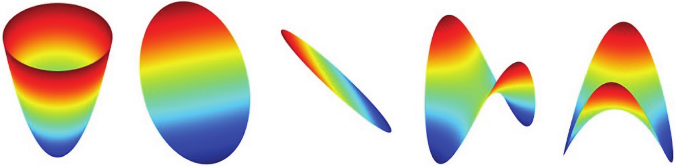
Opening image (of Steklov eigenfunctions) is courtesy of Chiu-Yen Kao.
Figure 1 is courtesy of Nsoki Mamie Mavinga.
Photo of Nsoki Mamie Mavinga is courtesy of Stephanie Specht.