My teenaged son's job requires him to deliver papers to 148 houses. When I deliver papers with him, we park my car, walk to each of the houses, and then return to the car. Naturally, we would like to choose the route that requires us to walk the shortest possible distance.
From one point of view, this is a pretty simple task: there are a finite number of routes so we could list them all and search through them to find the shortest. When we start to list all the routes, however, we find a huge number of them: 148!, to be precise, and
|
148!= |
2556323917872865588581178015776757943261545225324888777742656636831312 |
|
|
2650937538430929116102315575456544567283555639464949738814406570248083 |
|
|
3807378952671438814060814746021382234117929711163143053268084074819321 |
|
|
9035217998643200000000000000000000000000000000000 |
|
= |
2.55 $\cdot$ 10258. |
That looks like a big number. To put it in context, today's computers are able to perform about a billion operations every second, and the number of seconds in the life of the universe is about 1017. If we had been examining routes since the beginning of the universe, we would have considered only about 1026 of the possbilities; we couldn't honestly say we have even gotten started. Certainly, the newspaper's readers can't wait for us to find a solution this way.
Consider the same problem in a different context. Shown below are ten of my favorite places in Michigan:

If I would like to visit all of them and find the shortest possible route, I could examine the 10! = 3,628,800 possibilities and find this one:

The point is that even with a small number of sites to visit, the number of possible routes is very large and considerable effort is required to study them all.
The Traveling Salesman Problem
These problems are instances of what is known as the Traveling Salesman Problem. In both cases, we want to visit a number of sites using a route that minimizes the total distance traveled. More generally, we may wish to choose a route that minimizes some other quantity, such as the cost of the route.
I have described one way to find the optimal route by considering all of the possibilities, yet we intuitively feel that there must be a better way. Certainly, my son and I have found what we think is the best possible route through other means.
In fact, mathematicians have not been able to find a method for obtaining the optimal route in a general Traveling Salesman Problem that can be guaranteed to be significantly more efficient than this brute force technique in every instance. Simply said, this is a hard problem to solve in general. In this article, we'll explore why this is an interesting problem and describe a recent result concerning it.
After reading the two examples described above, you may start to see instances of the Traveling Salesman Problem all around you; for instance, how will you organize your day to go to work, the grocery store, take your kids to and from school, and stop by the coffee shop in the most efficient way. You can imagine that postal delivery services, like UPS and FedEx, face this problem when scheduling daily pickup and delivery of packages. Most likely, political campaigns try to minimize costs and maximize their candidate's exposure as they schedule campaign appearances around Iowa and New Hampshire.
William Cook's wonderful new book In Pursuit of the Traveling Salesman, describes many more instances of this problem, beginning with, well, traveling salesmen who need to visit a number of cities peddling a company's products. In addition, he explains more recent applications, from creating schedules for the efficient use of telescope time to new techniques for genome mapping.
As another example, when some digital circuit boards are produced, several thousand holes are drilled so that electronic components, such as resistors and integrated circuits, may be inserted. The machine that drills these holes must visit each of these locations on the circuit board and do it as efficiently as possible. Once again, the Traveling Salesman Problem.
Clearly, this problem is ubiquitous. We would like to have a good way to solve it.
How good is good?
As mentioned above, one way to solve a Traveling Salesman Problem (TSP) is to search through each of the possible routes for the shortest. If we have $n$ sites to visit, there are $n!$ possible routes, and this is an impossibly large number for even modest values of $n$, such as my son's paper route. When we consider the thousands of holes in an electronic circuit board, it is an understatement to say the problem is astronomically more difficult.
Mathematicians have developed a means of assessing the difficulty of a problem by measuring the complexity of any algorithm that solves the problem. Generally speaking, the complexity is a measure of how much effort is required to solve a problem as a function of the number of inputs into the problem, which we'll call $n$. For instance, we denote the complexity of our brute force algorithmic solution to the TSP by $O(n!)$, which we think of as roughly proportional to $n!$.
Suppose, for instance, that you would like to look up a number in the phone book. One way to do this is to start with "AAA Aardvarks" and proceed through the book, one entry at a time, until you find the one you're looking for. The effort here is proportional to $n$, the number of entries in the phone book, so we say that the complexity of this algorithm is $O(n)$. If the size of the phone book doubles, we have roughly twice as much work to do.
Of course, there's a better algorithm for finding phone numbers, a binary search algorithm in which you open the phone book in the middle, determine if the entry you're looking for comes before or after, and repeat. The effort required here is $O(\log(n))$, roughly proportional to the base 2 logarithm of $n$. In this case, if the size of the phone book doubles, you only need one more step. Clearly, this is a better algorithm.
Notice that the measure of complexity is associated to an algorithm that solves a problem, not the problem itself.
Now suppose that you have $n$ pairs of pants and $n$ shirts and that you consider each possible combination when you get dressed in the morning. Since there are $n^2$ combinations, the effort required is $O(n^2)$. If $n$ doubles, we need to do four times as much work.
We may now define an important class of problems, known as class P. A problem belongs to class P if there is an $O(n^k)$ algorithm that solves a problem for some power $k$. The P here stands for "polynomial"; the effort required to run the algorithm is proportional to a polynomial in $n$.
We generally think of class P problems as "easy" problems, even though the best algorithm available may be $O(n^k)$ for a high value of k. By comparison, our brute force algorithm for the TSP is $O(n!)$; if we increase $n$ by 1, we need to do $n$ times as much work.
At this time, we do not know if the TSP is in class P--that is, there is no known algorithm that solves a general TSP with polynomial complexity--but that doesn't mean that someone won't find one tomorrow.
A second class of problems is known as NP: a problem is NP if a potential solution can be checked by a polynomial-time algorithm; that is, the solution-checking algorithm is $O(n^k)$ for some $k$.
Generally speaking, it is easier to check a potential solution than it is to find solutions. For instance, finding the prime factors of 231,832,825,921 is challenging; checking that 233,021$\cdot$994,901 = 231,832,825,921 is relatively easy. Indeed, it follows that ${\bf P}\subset{\bf NP}$; that is, if we can generate solutions in polynomial time, we can verify that we have a solution in polynomial time as well.
Surprisingly enough, we do not know whether the TSP is in NP! Consider the special case of the Euclidean TSP: the sites here are taken to be in Euclidean space, and the cost to travel between sites is the Euclidean distance. If we fix a constant $K$, we may ask whether a route has a distance less than $K$. While this may seem like a simple question, answering it requires computing square roots and there is no known polynomial-time algorithm that can determine whether a sum of square roots is less than $K$!
Given this, it is tempting to think that class P problems are very special, and, in fact, we do know of problems that are not in P. However, there are no known problems that are in NP but not in P. It is therefore natural to ask whether ${\bf P}={\bf NP}$. This is one of the fundamental unresolved open questions in mathematics, and one of six questions whose answer is worth $1,000,000 from the Clay Mathematics Institute. You may read the official problem description here.
One final class of problems is NP-complete; a problem is in this class if any problem in NP can be reduced to the NP-complete problem in polynomial time. In spite of the fact that we do not know whether the TSP is in NP, we do know, remarkably, that it is NP-complete. Consequently, if you find a polynomial-time algorithm for the TSP, then we will know that ${\bf P}={\bf NP}$, and you will have earned $1,000,000.
In a poll conducted in 2002, Bill Gasarch asked a group of experts whether they believed that ${\bf P}={\bf NP}$ or not. Sixty-one believed that it was not true, and only nine thought it was. However, many believed that it would be a long time before we knew with certainty and that fundamentally new ideas were required to settle the question. You may read the results of this poll here.
It's easy to believe that ${\bf P}\neq{\bf NP}$; our experience is that it is typically easier to test potential solutions than it is to find solutions. However, the study of algorithms is relatively young, and one may imagine that, as the field matures, we will discover some fundamental new techniques that will show that these tasks require the same amount of effort. Perhaps we will be surprised with the kind of things we can easily compute.
What we do know
So the TSP feels like a hard problem, but we can't really be sure. Worse yet, we might not know for a long time. In the meantime, what have we learned about this problem?
Besides the brute-force $O(n!)$ algorithm, the best algorithm we currently have is an $O(n^2\cdot2^n)$ algorithm found by Held and Karp in 1962. Notice that this complexity is not polynomial given the presence of the exponential. This result has not been improved upon in 50 years.
However, new ideas have continually been found to attack the TSP that enable us to find optimal routes through ever larger sets of sites. In 1954, Dantzig, Fulkerson, and Johnson used linear programming to find the shortest route through major cities in (then) all 48 states plus the District of Columbia. Since that time, optimal routes have been found through 3038 cities (in 1992), 13,509 (in 1998), and 85,900 in 2006. The computer code used in some of these calculations is called Concorde and is freely available.
A striking example is the nearly optimal TSP route through 100,000 sites chosen so as to reproduce Leonardo da Vinci's Mona Lisa.
Remember that the general TSP is defined by some measurement of the cost of a trip between different sites. Perhaps the general TSP is hard to solve but perhaps better algorithms can be found for special cases of the TSP, such as the Euclidean TSP, which is also known to be NP-complete. In fact, we will now look at a result about the Euclidean TSP that may shed some light on the ${\bf P}={\bf NP}$ question.
Polynomial Time Approximation Schemes
Perhaps if a job is too hard to complete, we would be satisfied with almost finishing it. That is, if we cannot find the absolute shortest TSP route, perhaps we can find a route that we can guarantee is no more than 10% longer than the shortest route or perhaps no more than 5% longer.
In 1976, Christofides found a polynomial-time algorithm that produced a route guaranteed to be no more than 50% longer than the optimal route. But the question remained: if we fix a tolerance, is there a polynomial-time algorithm that will find a route whose length is within the given tolerance of the optimal route.
In the mid 1990's, Arora and Mitchell independently found algorithms that produce approximate solutions to the Euclidean TSP in polynomial time. Arora created an algorithm that, given a value of $c>1$, finds a route whose length is no more than $1+1/c$ times the shortest route. The complexity of a randomized version of his algorithm, which we will describe now, is $O(n(\log n)^{O(c)})$.
Arora's algorithm applies dynamic programming to a situation created by a data structure known as a quadtree. To begin, consider the locations that we are to visit in our Euclidean TSP and put them inside a square.

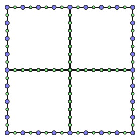
For the time being, let's focus on the square and subdivide it to obtain four squares.

Continuing this process creates a quadtree; every node in the tree is a square and internal nodes have four children. The root of the tree is the initial square.

Now we can get started describing Arora's algorithm to find approximate solutions to the TSP. We fix a number $c$ and look for a route whose length is no more than $1+1/c$ times the optimal route. For instance, if $c=10$, then we will find a route whose length is no more than 10% longer than the optimal route.
We will construct a quadtree so that each leaf contains a single location in our TSP. If two locations are very close together, our tree may have to descend relatively deep in the tree to find squares that separate the two points. To avoid this, we will perturb the points slightly: if the side of the original bounding box has length $L$, we construct a grid of width $L/(8nc)$ and move each location to its nearest grid point.


Let's make two observations: suppose that $OPT$ is the length of the optimal route. Since $L$ is the side of the bounding box of the locations, we have $OPT\geq 2L$. Second, notice that the distance each point is moved by less than $L/(8nc)$, which means that the total length of any route will change by at most $2n\cdot L/(8nc) < OPT/(4c)$. Since we are looking for a route whose length is no more than $OPT/c$ longer than the optimal route, this is an acceptable perturbation.
Though two sites may be moved to the same grid point, we may otherwise guarantee that the sites are separated by a distance of at least $L/(8nc)$. We now construct a quadtree by subdividing squares when there is more than one point within the square.

Due to our perturbation, the depth of the quadtree is now $O(\log n)$ so the number of squares in the quadtree is $T=O(n\log n)$.
We may also rescale the plane to assume that the sites have integral coordinates. This does not affect the relative lengths of routes and will pay off later.
Next we will describe a dynamic programming algorithm to find an approximate solution to our TSP. In each square, we will restrict the points at which routes may enter that square. To this end, we choose an integer $m$, a power of 2 in the range $[c\log L, 2c\log L]$. On the side of each square, we place $m+1$ equally spaced points, called portals.

The motivation for introducing portals is so that we need only examine a relatively small number of locations at which a path may enter a square. The more portals we have, the closer our route will be to optimal.
Since $m$ is a power of 2, the portals of an internal node are also portals for each of its children.
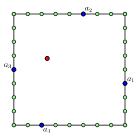
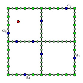
On each square, we now consider the multipath problem given by specifying a collection of portals $a_1$, $a_2$, $a_3$, ..., $a_{2p}$. We ask to find the shortest collection of paths that connect $a_1$ to $a_2$, $a_3$ to $a_4$, and so on, and that visit each TSP site inside the square.
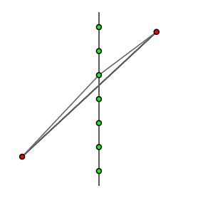
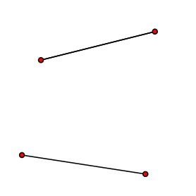
For the leaves, this is a relatively simple task; we list all the possible paths and find the shortest one. For the problem above, there are only two possibilities:


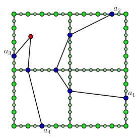
and the shortest collection of paths, the solution to the multipath problem, is the one on the right. For each collection of portals $a_1,a_2,\ldots, a_{2p}$, we keep a record of this solution.
For internal nodes, we may have a multipath problem like this:
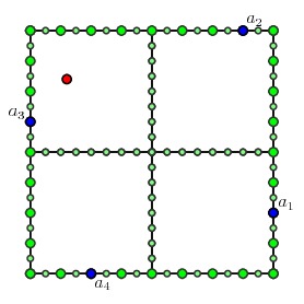
We assume that we have already solved all possible multipath problems for the children. To solve the multipath problem for the internal node, we consider each possible choice of portals on the inner edges of the children that could produce a multipath.
Now we look up the solutions of the multipath problems on the children to construct the multipath on the parent node.
In this way, we only need to search over all the choices for portals on the inner edges to find the solution to the multipath problem in the parent node.
We work our way up the tree until we are at the root, at which point we solve the multipath problem with no portals on the boundary. This gives a route that is a candidate for our approximate solution to the TSP.
To estimate the computation effort required to run this algorithm, we need to remember that there are $T = O(n\log n)$ squares in the quadtree. With some care, we may enumerate the choices of portals for which we must solve the multipath problem, which leads to Arora's estimate of the complexity as $O(n(\log n)^{O(c)})$.
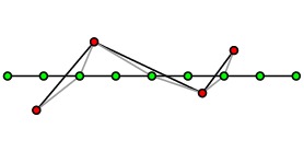
The route we find may have crossings, but we may eliminate crossings without increasing the length of the route.

Now it turns out that the algorithm, as stated above, may not produce a route approximating the TSP solution with the desired accuracy. For instance, this may happen when the route crosses a square in the quadtree many times.
Therefore, Arora introduces a shifted quadtree obtained by translating the squares in the quadtree and allowing them to "wrap around," if necessary.

Arora analyzes the effect that these shifts have on the number of times that the route produced by the algorithm crosses the sides of squares. This analysis shows that if a shift is chosen at random, then the probability is at least 1/2 that the route found by the algorithhm has a length less than $(1+1/c)OPT$ and is therefore within our desired tolerance.
To guarantee that we obtain a route within the desired tolerance, we may run through every possible shift and simply take the shortest of these routes. Assuming that the sites have integral coordinates, we only need to consider $L^2$ shifts, which increases the running time by a factor of $L^2=O(n^2)$, so that the algorithm still completes in polynomial-time.
Summary
As implementations of Arora's algorithm are not particularly efficient, we should view this result primarily as a theoretical one.
Remember that the Euclidean TSP is NP-complete; this means that if we can find a polynomial time algorithm that solves the Euclidean TSP, then ${\bf P}={\bf NP}$. Arora's result doesn't prove this; however, it is remarkable for it shows that we may approximate the optimal route to any desired accuracy with a polynomial-time algorithm. The problem is that we have to work harder and harder when we ask for greater accuracy.
Both Arora and Mitchell were awarded the Gödel Prize of the Association of Computing Machinery in 2010 in recognition of the significance of their results.
References
There has been a great deal written about the TSP and ${\bf P}$ versus ${\bf NP}$. Included below are references I found helpful in preparing this article.
-
Sanjeev Arora, Polynomial Time Approximation Schemes for Euclidean Traveling Salesman and other Geometric Problems, Journal of the Association of Computing Machinery, 45(5), 753-782.
-
Joseph S.B. Mitchell, Guillotine subdivisions approximate polygonal subdivisions: A simple polynomial-time approximation scheme for the geometric TSP, k-MST, and related problems, SIAM Journal of Computing, 28(4), 1298-1309.
-
William J. Cook, In Pursuit of the Traveling Salesman, Princeton University Press, 2012.
Written in an engaging, personal style, this highly readable book includes a great deal of history and anecdotes surrounding the TSP as well an introduction to techniques and results.
-
E.L. Lawler, J.K. Lenstra, A.H.G. Rinnooy Kan, D.B.Shmoys, The Traveling Salesman Problem, John Wiley & Sons, 1985.
-
David L. Applegate, Robert E. Bixby, Vasek Chvatal, William J. Cook, The Traveling Salesman Problem: A Computational Study, Princeton University Press, 2006.
-
The Traveling Salesman Problem.
This site, maintained by William Cook, will be of use to anyone interested in the TSP.

 David Austin