Using Projective Geometry to Correct a Camera
There's nothing particularly deep in this problem or the solution, but I hope that it demonstrates some of the pleasure to be found in using one's mathematical intuition...
Introduction
Not long ago, I received a call from an engineer working in the automotive industry who needed to correct the image produced by a camera that was improperly aligned. As it happened, I had read one of Jim Blinn's computer graphics columns within the past week and saw that it explained a simple and elegant solution to the problem.
In this column, I will describe the problem and then show how the ideas in Blinn's column provided a solution. There's nothing particularly deep in this problem or the solution, but I hope that it demonstrates some of the pleasure to be found in using one's mathematical intuition.
First, the problem. The engineering company was building a new automotive suspension system and using a camera to measure the motion of a tire connected to the suspension system in their test lab. The camera would track the motion of the tire by periodically recording the location of certain points on the tire.
Obtaining the accuracy needed for their tests required the camera to be precisely aligned in a plane parallel to that of the tire; in practice, this was difficult to achieve.
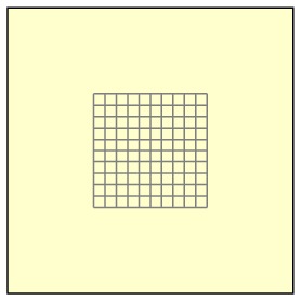
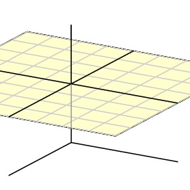
Here's a simplified version of the problem. Suppose you'd like to take a picture of this plane,

which sits in three-dimensional space.

If the camera is perfectly aligned with the plane,

then the image will be uniformly scaled but otherwise faithfully recorded.
However, if the plane of the camera is not parallel to the plane of the image,
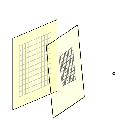
then the image will distort the plane.
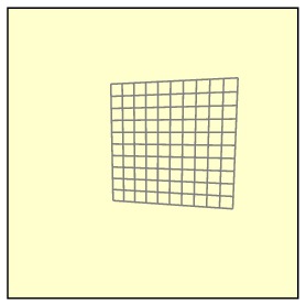
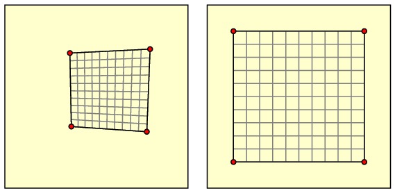
Our goal is to take the distorted image recorded by the camera, as shown on the left, and reconstruct the original image as if the camera were properly aligned, as on the right.
Projective transformations
To begin, we will describe the function that projects one plane onto another. It does not matter if we consider the projection of the plane onto the camera's plane or the inverse projection from the camera onto the original plane.

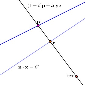
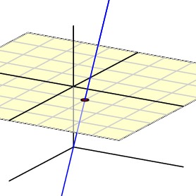
Suppose we project the point ${\bf p}$ onto the plane described by the equation ${\bf n}\cdot {\bf x} = C$. The following figure shows a two-dimensional version of this problem.

We will parametrize the points on the line from ${\bf p}$ to the eye by ${\bf r} = (1-t){\bf p} + t{\bf eye}$ and ask when this point lies on the plane ${\bf n}\cdot {\bf x} = C$.

This gives a condition on $t$ from which we find $$ t = \frac{C-{\bf n}\cdot {\bf p}}{{\bf n}\cdot{\bf eye} -{\bf n}\cdot {\bf p}}, $$
and therefore $$ {\bf r} = \frac{{\bf n}\cdot{\bf eye} - C}{{\bf n}\cdot{\bf eye}-{\bf n}\cdot {\bf p}} {\bf p} + \frac{C- {\bf n}\cdot{\bf p}}{{\bf n}\cdot{\bf eye} - {\bf n}\cdot{\bf p}} {\bf eye} $$
If we assume there are coordinates on the planes, we find the function has the form $$ (x,y)\mapsto(u,v) = \left(\frac{ax+by+c}{gx + hy + j}, \frac{dx + ey + f}{gx+hy+j}\right). $$
Given our two images, we will choose four points in the distorted image and four corresponding points in the corrected image, and from this data, we will reconstruct the function.
The form of this function, known as a projective transformation, is tantalizing; though the components are rational functions, the numerators and denominators are simply linear. For this reason, it is natural to recast this function as a transformation of the projective plane, the set of lines in ${\bf R}^3$ passing through the origin.

By placing the Euclidean plane inside ${\bf R}^3$ as the plane $z=1$,
we see that the Euclidean plane sits inside the projective plane since a line intersects the plane $z=1$ in at most one point.
Points in the projective plane are described using homogeneous coordinates, by which we denote a line in the projective plane as $[x,y,z]$ where $(x,y,z)$ is a point on the line. Notice that any scalar multiple of $(x,y,z)$ is also a point on this line, which means that the homogeneous coordinate is only defined up to a scalar multiple. That is, $[x,y,z] = [wx,wy,wz]$.
Notice that the points in the Euclidean plane have the form $[x,y,1]$. The other points in the projective plane have the form $[x,y,0]$ and correspond to lines lying in the $xy$-plane. These points are sometimes referred to as "at infinity" because such a point is the limit of an unbounded sequence of points in the Euclidean plane.
If we adopt homogeneous coordinates, we may write our transformation in the form $$ [x,y,1]\mapsto [u,v,1] = [ax+by+c, dx+ey+f, gx+hy+j], $$
whose linearity will prove convenient. Determining the transformation requires us to determine the matrix formed by the constants $a, b,\ldots, j$. This matrix, however, is only defined up to a scalar multiple due to the use of homogeneous coordinates.
Comments?
A naive solution
Our problem is not especially difficult as it admits a straightforward solution, which we will now describe.
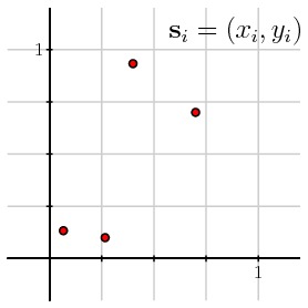
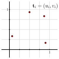
The image on the left is called the source space while that on the right is the target space. We are given four points ${\bf s}_i = (x_i, y_i)$ in the source space and their four images ${\bf t}_i=(u_i, v_i)$ under the transformation in the target space. Our goal is to determine the transformation.

We have $$ \left[x_i \quad y_i \quad 1 \right] \left[\begin{array}{ccc} a & d & g \\ b & e & h \\ c & f & j \end{array} \right] = w_i\left[u_i \quad v_i \quad 1\right], $$
where $w_i=gx_i + hy_i + j$ is a scaling factor. In other words, \[ \begin{eqnarray*} ax_i + by_i + c & = & w_i u_i \\ dx_i + ey_i + f & = & w_i v_i \\ gx_i + hy_i + j & = & w_i \end{eqnarray*} \]
or \[ \begin{eqnarray*} ax_i + by_i + c & = & (gx_i+hy_i + j) u_i \\ dx_i + ey_i + f & = & (gx_i+hy_i + j) v_i \end{eqnarray*} \]
or \[ \begin{eqnarray*} x_ia + y_ib + c -x_i u_i g - y_i u_i h - u_i j & = & 0 \\ x_id + y_ie + f -x_i v_i g - y_i v_i h - v_i j & = & 0 \end{eqnarray*} \]
or \[\left[ \begin{array}{ccccccccc} x_i & y_i & 1 & 0 & 0 & 0 & -x_i u_i & - y_i u_i & - u_i \\ 0 & 0 & 0 & x_i & y_i & 1 & -x_i v_i & - y_i v_i & - v_i \end{array} \right] \left[\begin{array}{c} a \\ b \\ c \\ d \\ e \\ f \\ g \\ h \\ j \end{array} \right] = \left[ \begin{array}{c} 0 \\ 0 \end{array} \right]. \]
With four pairs of points $\{{\bf s}_i\}$ and $\{{\bf t}_i\}$, we obtain an $8\times 9$ homogeneous system of equations that will determine the constants $a,b,\ldots,j$ up to a scalar multiple. This explains why we need four points to determine the transformation.
The resulting transformation is denoted by ${\bf M_{st}}$ and defined by the matrix $$ {\bf M_{st}} = \left[\begin{array}{ccc} a & d & g \\ b & e & g \\ c & f & j \end{array}\right]. $$
This is the obvious solution to the problem. Computationally, it is somewhat unpleasant to solve an $8\times9$ system, but it is not too difficult. The most serious complaint may be that we have lost sight of any geometric intuition we had into the problem.
Comments?
Doing the two-step
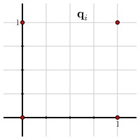
A more interesting solution was proposed by Paul Heckbert. Rather than finding the transformation that converts the points ${\bf s}_i$ directly into ${\bf t}_i$, let's construct a two-step process with an intermediate set of points ${\bf q}_i$, the vertices of the unit square. That is, we will map
|
${\bf s}_i$ |
$\mapsto$ |
${\bf q}_i$ |
$\mapsto$ |
${\bf t}_i$ |
 |
|
 |
|
 |
We define transformations ${\bf M_{sq}}$ and ${\bf M_{qt}}$ such that ${\bf s}_i{\bf M_{sq}}={\bf q}_i$ and ${\bf q}_i{\bf M_{qt}} = {\bf t}_i$. Our ultimate goal is the composition $$ {\bf M_{st}} = {\bf M_{sq}} {\bf M_{qt}}. $$
Notice, however, that ${\bf M_{sq}} = {\bf M^{-1}_{qs}}$ and finding ${\bf M_{qs}}$ is fundamentally the same task as finding ${\bf M_{qt}}$.
Heckbert's idea is helpful because the coordinates of the vertices of the unit square have lots of zeroes: $(0,0)$, $(1,0)$, $(1,1)$, and $(0,1)$, which leads to much simpler equations. For instance, since ${\bf q}_0 = (0,0)$, two of the equations are \[\left[ \begin{array}{ccccccccc} 0 & 0 & 1 & 0 & 0 & 0 & 0 & 0 & - u_0 \\ 0 & 0 & 0 & 0 & 0 & 1 & 0 & 0 & - v_0 \end{array} \right] \left[\begin{array}{c} a \\ b \\ c \\ d \\ e \\ f \\ g \\ h \\ j \end{array} \right] = \left[ \begin{array}{c} 0 \\ 0 \end{array} \right]. \]
In fact, Blinn shows how to solve these eight equations explicitly in terms of the coordinates ${\bf t}_i = (u_i, v_i)$ to find the transform ${\bf M_{qt}}$. The solution isn't particuarly pretty, but relatively little computational effort is required.
We then have \[\begin{eqnarray*} {\bf M_{st}} & = & {\bf M_{sq}} {\bf M_{qt}} \\ & = & {\bf M^{-1}_{qs}} {\bf M_{qt}}. \\ \end{eqnarray*} \]
Since we may multiply the matrix ${\bf M_{st}}$ by a scalar and obtain the same projective transformation, we may replace ${\bf M^{-1}_{qs}}$ by the adjoint ${\bf M^*_{qs}}$, which differs from the inverse by multiplying by the determinant of ${\bf M_{qs}}$. This leaves us with $$ {\bf M_{st}} = {\bf M^*_{qs}} {\bf M_{qt}}. $$
Comments?
Barycentric coordinates
Blinn also describes a second method for solving this problem found by Kirk Olynyk, a colleague at Microsoft Research, who used barycentric coordinates to simplify the computations. We will first describe barycentric coordinates and then Olynyk's method.
If we have three non-collinear points in the plane ${\bf p}_0$, ${\bf p}_1$, and ${\bf p}_2$, we may uniquely represent any point ${\bf p}$ in the plane in the form $$ {\bf p} = \pi_0 {\bf p}_0 + \pi_1 {\bf p}_1 + \pi_2 {\bf p}_2, $$
with the additional condition that $\pi_0+\pi_1+\pi_2 = 1$. This is seen easily enough when one of the ${\bf p}_i$ is the origin. The more general case follows by applying a uniform translation to all four points.
If we apply this to a point in our target space, we have \[ \begin{eqnarray*} \tau_0 {\bf t}_0 + \tau_1 {\bf t}_1 + \tau_2 {\bf t}_2 & = & {\bf t} \\ \left[\begin{array}{ccc} \tau_0 & \tau_1 & \tau_2 \end{array}\right] \left[\begin{array}{ccc} u_0 & v_0 & 1 \\ u_1 & v_1 & 1 \\ u_2 & v_2 & 1 \\ \end{array} \right] & = & \left[\begin{array}{ccc} u & v & 1 \end{array}\right], \end{eqnarray*} \]
and similarly for a point in the source space: $$ \sigma_0 {\bf s}_0 + \sigma_1 {\bf s}_1 + \sigma_2 {\bf s}_2 = {\bf s}. $$
Let's now consider the effect of our transformation ${\bf M_{st}}$ on the barycentric coordinates. \[\begin{eqnarray*} w{\bf t} & = & {\bf s}{\bf M_{st}} \\ w \left[\begin{array}{ccc} \tau_0 & \tau_1 & \tau_2 \end{array}\right] \left[\begin{array}{ccc} u_0 & v_0 & 1 \\ u_1 & v_1 & 1 \\ u_2 & v_2 & 1 \\ \end{array} \right] & = & \left[\begin{array}{ccc} \sigma_0 & \sigma_1 & \sigma_2 \end{array}\right] \left[\begin{array}{ccc} x_0 & y_0 & 1 \\ x_1 & y_1 & 1 \\ x_2 & y_2 & 1 \\ \end{array} \right]{\bf M_{st}} \\ \left[\begin{array}{ccc} w\tau_0 & w\tau_1 & w\tau_2 \end{array}\right] \left[\begin{array}{ccc} u_0 & v_0 & 1 \\ u_1 & v_1 & 1 \\ u_2 & v_2 & 1 \\ \end{array} \right] & = & \left[\begin{array}{ccc} \sigma_0 & \sigma_1 & \sigma_2 \end{array}\right] \left[\begin{array}{ccc} w_0u_0 & w_0v_0 & w_0 \\ w_1u_1 & w_1v_1 & w_1 \\ w_2u_2 & w_2v_2 & w_2 \\ \end{array} \right] \\ \left[\begin{array}{ccc} w\tau_0 & w\tau_1 & w\tau_2 \end{array}\right] \left[\begin{array}{ccc} u_0 & v_0 & 1 \\ u_1 & v_1 & 1 \\ u_2 & v_2 & 1 \\ \end{array} \right] & = & \left[\begin{array}{ccc} w_0\sigma_0 & w_1\sigma_1 & w_2\sigma_2 \end{array}\right] \left[\begin{array}{ccc} u_0 & v_0 & 1 \\ u_1 & v_1 & 1 \\ u_2 & v_2 & 1 \\ \end{array} \right] \\ \end{eqnarray*} \]
showing that $$ \left[\begin{array}{ccc} w\tau_0 & w\tau_1 & w\tau_2 \end{array}\right] = \left[\begin{array}{ccc} w_0\sigma_0 & w_1\sigma_1 & w_2\sigma_2 \end{array}\right] $$
This shows that the effect of the transformation ${\bf M_{st}}$ on barycentric coordinates is simple multiplication: $w\tau_i = w_i\sigma_i$. Once we determine the constants $w_0$, $w_1$, and $w_2$, we may find $w$ using the requirement that $\tau_0+\tau_1+\tau_2 = 1$.
How then do we determine $w_0$, $w_1$, and $w_2$? Remember that we have a fourth pair of points ${\bf s}_3$ and ${\bf t}_3$ and that ${\bf s}_3{\bf M_{st}} = {\bf t}_3$. If we write the barycentric coordinates for ${\bf s}$ as $[\tilde{\sigma}_0 \quad \tilde{\sigma}_1\quad\tilde{\sigma}_2]$ and the barycentric coordinates of ${\bf t}$ as $[\tilde{\tau}_0 \quad \tilde{\tau}_1\quad\tilde{\tau}_2]$, then we have, up to a scaling constant, $$ w_i = \frac{\tilde{\tau}_i}{\tilde{\sigma}_i}. $$
In other words, in barycentric coordinates, the transformation ${\bf M_{st}}$ is simply given by the diagonal matrix $$ w[\tau_0 \quad \tau_1 \quad \tau_2] = [\sigma_0 \quad \sigma_1\quad \sigma_2] \left[ \begin{array}{ccc} \frac{\tilde{\tau}_0}{\tilde{\sigma}_0} & 0 & 0 \\ 0 & \frac{\tilde{\tau}_1}{\tilde{\sigma}_1} & 0 \\ 0 & 0 & \frac{\tilde{\tau}_2}{\tilde{\sigma}_2} \\ \end{array}\right]. $$
where $\tilde{\sigma}_i$ and $\tilde{\tau}_i$ are the barycentric coordinates of ${\bf s}_3$ and ${\bf t}_3$, respectively.
This is an especially simple expression for ${\bf M_{st}}$. Notice, however, that there is some additional work required in finding the barycentric coordinates of ${\bf s}$ through \[\begin{eqnarray*} [\sigma_0 \quad \sigma_1 \quad \sigma_2] \left[\begin{array}{ccc} x_0 & y_0 & 1 \\ x_1 & y_1 & 1 \\ x_2 & y_2 & 1 \\ \end{array}\right] & = & [x \quad y \quad 1 ] \\ [\sigma_0 \quad \sigma_1 \quad \sigma_2] & = & [x \quad y \quad 1 ] \left[\begin{array}{ccc} x_0 & y_0 & 1 \\ x_1 & y_1 & 1 \\ x_2 & y_2 & 1 \\ \end{array}\right]^{-1} \end{eqnarray*} \]
and then recovering the target point ${\bf t}$ from its barycentric coordinates.
To summarize, the transformation ${\bf s}\mapsto{\bf t}$ is constructed by
-
finding the barycentric coordinates of ${\bf s}$,
-
computing $w\tau_i = (\tilde{\tau}_i/\tilde{\sigma}_i) ~ \sigma_i$,
-
normalizing the coordinates so that $\tau_0+\tau_1+\tau_2 = 1$,
-
and reconstructing ${\bf t}$ from its barycentric coordinates.
Olynyk's method is similar in spirit to Heckbert's in that both use an intermediate step in finding the transformation ${\bf M_{st}}$. Heckbert's process decomposes ${\bf M_{st}}$ into two transformations taking us through a standard set of points, the vertices of the unit square. Olynyk's process decomposes ${\bf M_{st}}$ by first converting to barycentric coordinates, which are then individually scaled.
Comments?
Blinn's final improvement
Blinn found a third method, based on the work of Heckbert and Olynyk, whose simplicity is stunning. We will follow Heckbert's approach of factoring ${\bf M_{st}}$ through an intermediate set of points ${\bf b}_i$. Rather than using the unit square, however, we will choose the points in the projective plane to have the largest possible number of zeroes: \[\begin{eqnarray*} {\bf b}_0 & = & [1\quad 0 \quad0] \\ {\bf b}_1 & = & [0\quad 1 \quad0] \\ {\bf b}_2 & = & [0\quad 0 \quad1] \\ {\bf b}_3 & = & [1\quad 1 \quad1] \\ \end{eqnarray*} \]
Notice that two of these points lie at infinity, but why should we object? To describe the transformation ${\bf M_{bt}}$, notice that ${\bf b}_i {\bf M_{bt}} = {\bf t}_i = [w_i u_i\quad w_iv_i\quad w_i].$ Considering the first three points ${\bf b}_0$, ${\bf b}_1$, and ${\bf b}_2$, we find \[ \left[\begin{array}{ccc} 1 & 0 & 0 \\ 0 & 1 & 0 \\ 0 & 0 & 1 \\ \end{array}\right] {\bf M_{bt}} = \left[\begin{array}{ccc} w_0u_0 & w_0v_0 & w_0 \\ w_1u_1 & w_1v_1 & w_1 \\ w_2u_2 & w_2v_2 & w_2 \\ \end{array}\right]. \]
From this, we immediately see that transformation ${\bf M_{bt}}$: $${\bf M_{bt}} = \left[\begin{array}{ccc} w_0u_0 & w_0v_0 & w_0 \\ w_1u_1 & w_1v_1 & w_1 \\ w_2u_2 & w_2v_2 & w_2 \\ \end{array}\right] = \left[\begin{array}{ccc} w_0 & 0 & 0 \\ 0 & w_1 & 0 \\ 0 & 0 & w_2 \\ \end{array}\right] \left[\begin{array}{ccc} u_0 & v_0 & 1 \\ u_1 & v_1 & 1 \\ u_2 & v_2 & 1 \\ \end{array}\right]. $$
All that's required now is to find $w_0$, $w_1$, and $w_2$, which we may do using the fourth point: \[ \begin{eqnarray*} {\bf b}_3{\bf M_{bt}} & = & {\bf t}_3 \\ [1\quad1\quad1] \left[\begin{array}{ccc} w_0 & 0 & 0 \\ 0 & w_1 & 0 \\ 0 & 0 & w_2 \\ \end{array}\right] \left[\begin{array}{ccc} u_0 & v_0 & 1 \\ u_1 & v_1 & 1 \\ u_2 & v_2 & 1 \\ \end{array}\right] & = & [w_3u_3 \quad w_3v_3 \quad w_3] \\ [w_0\quad w_1\quad w_2] & = & w_3[u_3 \quad v_3 \quad 1] \left[\begin{array}{ccc} u_0 & v_0 & 1 \\ u_1 & v_1 & 1 \\ u_2 & v_2 & 1 \\ \end{array}\right]^{-1} \end{eqnarray*} \]
Here we see a clear relationship with Olynyk's method: $w_0$, $w_1$ and $w_2$ are simply the barycentric coordinates of ${\bf t}_3$ scaled by $w_3$. $$ [w_0\quad w_1\quad w_2] = w_3[\tilde{\tau}_0\quad \tilde{\tau}_1\quad \tilde{\tau}_2]. $$
Since ${\bf M_{bt}}$ is only defined up to a multiplicative constant, we may choose $w_3$ to be anything we wish. If we choose $$ w_3 = \det \left[\begin{array}{ccc} u_0 & v_0 & 1 \\ u_1 & v_1 & 1 \\ u_2 & v_2 & 1 \\ \end{array}\right], $$
then we arrive at $$ [w_0\quad w_1 \quad w_2] = [u_3 \quad v_3 \quad 1] \left[\begin{array}{ccc} u_0 & v_0 & 1 \\ u_1 & v_1 & 1 \\ u_2 & v_2 & 1 \\ \end{array}\right]^* $$
Using the target data, we will define the matrix ${\bf T}$ by $$ {\bf T} = \left[\begin{array}{ccc} u_0 & v_0 & 1 \\ u_1 & v_1 & 1 \\ u_2 & v_2 & 1 \\ \end{array}\right], $$
so that $$ [w_0\quad w_1 \quad w_2] = [u_3 \quad v_3 \quad 1] \quad {\bf T}^* $$
Of course, we still have to find ${\bf M_{sb}}$ in a similar way: $$ {\bf M_{bs}} = \left[\begin{array}{ccc} z_0 & 0 & 0 \\ 0 & z_1 & 0 \\ 0 & 0 & z_2 \\ \end{array}\right] {\bf S}, $$
where $$ [z_0\quad z_1 \quad z_2] = [x_3 \quad y_3 \quad 1]\quad {\bf S}^* $$
and ${\bf S}$ is the matrix formed by the target data: $${\bf S} = \left[\begin{array}{ccc} x_0 & y_0 & 1 \\ x_1 & y_1 & 1 \\ x_2 & y_2 & 1 \\ \end{array}\right]. $$
Putting everything together, we arrive at \[\begin{eqnarray*} {\bf M_{st}} & = &{\bf M_{sb}}{\bf M_{bt}} \\ & = & {\bf M_{bs}^*} {\bf M_{bt}} \\ & = & S \left[\begin{array}{ccc} z_0 & 0 & 0 \\ 0 & z_1 & 0 \\ 0 & 0 & z_2 \\ \end{array}\right]^* \left[\begin{array}{ccc} w_0 & 0 & 0 \\ 0 & w_1 & 0 \\ 0 & 0 & w_2 \\ \end{array}\right]{\bf T}^* \\ & = & {\bf S} \left[\begin{array}{ccc} w_0z_1z_2 & 0 & 0 \\ 0 & z_0w_1z_2 & 0 \\ 0 & 0 & z_0z_1w_2 \\ \end{array}\right]{\bf T}^*. \end{eqnarray*} \]
To top it off, Blinn gives a simple geometric interpretation to $w_i$ and $z_i$. Recall that \[ \begin{eqnarray*} [w_0\quad w_1 \quad w_2] & = & [u_3 \quad v_3 \quad 1] \left[\begin{array}{ccc} u_0 & v_0 & 1 \\ u_1 & v_1 & 1 \\ u_2 & v_2 & 1 \\ \end{array}\right]^* \\ & = & [u_3 \quad v_3 \quad 1] \left[\begin{array}{ccc} v_1-v_2 & v_2-v_0 & v_0-v_1 \\ u_2-u_1 & u_0-u_2 & u_1-u_0 \\ u_1v_2-u_2v_1 & u_2v_0-u_0v_2 & u_0v_1-u_1v_0 \\ \end{array}\right], \end{eqnarray*} \]
which shows that \[\begin{eqnarray*} w_0 & = &(u_1-u_3)(v_2-v_3) - (u_2-u_3)(v_1-v_3) \\ w_1 & = &(u_2-u_3)(v_0-v_3) - (u_0-u_3)(v_2-v_3) \\ w_2 & = &(u_0-u_3)(v_1-v_3) - (u_1-u_3)(v_0-v_3). \end{eqnarray*} \]
These expressions demonstrate that $w_i$ may be interepreted as twice the signed area of one of the triangles formed by the points ${\bf t}_i$. In the following figures, green represents a positive area while red represents a negative area.


Comments?
Summary
It's hard to imagine a simpler expression for ${\bf M_{st}}$: $$ {\bf M_{st}} = {\bf S} \left[\begin{array}{ccc} w_0z_1z_2 & 0 & 0 \\ 0 & z_0w_1z_2 & 0 \\ 0 & 0 & z_0z_1w_2 \\ \end{array}\right]{\bf T}^*. $$
Remembering that ${\bf S}$ is formed from the source data ${\bf s}_i$ and ${\bf T}$ from the target data ${\bf t}_i$, we need only compute the $w_i$ and $z_i$, which is, as shown above, a simple task.
As we have seen, we may find ${\bf M_{st}}$ by solving an $8\times9$ homogeneous system of equations. However, by considering the geometric nature of the problem, Heckbert, Olynyk, and Blinn each found increasingly simple forms for ${\bf M_{st}}$.
References

 David Austin