Sums and Integrals: The Swiss analysis knife
The charm of the formula discovered by him [Euler] and MacLaurin is that it applies to a remarkable assortment of mathematical questions...
 Bill Casselman
University of British Columbia, Vancouver, Canada
Email Bill Casselman
Introduction
In the early 18th century the Scottish mathematician Colin MacLaurin and the Swiss mathematician Leonhard Euler discovered, almost simultaneously and apparently quite independently, a rather strange formula relating the integral of a function over an interval spanned by integers $k$, $\ell$ and the sum of $f(n)$ over the integers in that interval. Euler has left a detailed record of how he came to it--he was largely motivated by problems involving efficient computation of infinite series that did not obviously allow of efficient computation. For most of the series he wanted to compute there are now better methods known, but the charm of the formula discovered by him and MacLaurin is that it applies to a remarkable assortment of mathematical questions. It is a kind of universal tool. The original formula applied only to functions of one variable, but in recent years there has been much research into analogous formulas involving functions of several variables, and indeed this is still an active and interesting area of investigation, with connections to a wide range of fields of mathematics including number theory, topology, and geometry. Besides, even in dimension one there seem to remain a few puzzles concerning exactly what functions the formula applies to, and how it is to be interpreted.
There is already a large literature on this topic, both in publications and on the Internet. But the summation formula of Euler and MacLaurin is beautiful enough to warrant yet another.
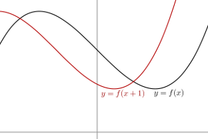
If $f$ is any function of a real variable and $t$ is a real number, one may define the shift operator $R_{t}f$ by the formula $$ [R_{t}f](x) = f(x+t) \, . $$ Its effect on the graph of $f$ is that it shifts it a distance $t$ to the left.
Then, at least formally, the expression of $f$ in terms of its Taylor series says that $$ [R_{t}f](x) = f(x) + t\cdot f'(x) + t^{2} \cdot { f''(x) \over 2 } + t^{3} \cdot {f^{(3)}(x) \over3! } + \cdots $$ It may happen that this infinite series does not in fact make any obvious sense, but if $f(x)$ is a polynomial then all but a finite number of terms vanish and the equation is valid.
Let $D$ be the differentiation operator $d/dx$. Thus $D^{n}f = f^{(n)}$. One may define, again at least formally, a family of new operators by the formula $$ e^{tD} = I + t\cdot D + t^{2}\cdot { D^{2} \over 2 } + t^{3} \cdot { D^{3} \over 3! } + \cdots $$ What we have seen is that $e^{tD}$ and $R_{t}$ agree on polynomials. Consequently $$ [(e^{D} - I)f](x) = [\Delta f](x) = f(x+1) - f(x) \, . $$ or $$ \Delta = e^{D} - I $$ as operators on polynomials.
Suppose now that we want to solve a difference equation $$ \Delta F = f $$ where $f$ is a polynomial restricted to the integers. (We shall see an interesting example in just a moment.) Adding a constant to a solution gives also a solution, so we may as well assume the initial condition $F(0) = 0$.
There are two ways to describe the solution. The first is straightforward but unenlightening: $$ F(n) = \cases { f(0) + f(1) + \cdots + f(n-1) \phantom{xxxx} & $n \gt 0$ \cr \phantom{xxxxxxxxxxxx} 0 & $n = 0$ \cr -f(-1) - f(-2) - \cdots - f(n) & $n \lt 0$. \cr } $$ Why unenlightening? Say $f(n) = n^{k}$. Then for $n > 0$ $$ F(n) = 1 + 2^{k} + 3^{k} + \cdots + (n-1)^{k} \, . $$ In other words, we are looking for a formula for the sum of the first $n$ non-negative integral $k$-th powers. As for the second description, we can write our equation as $$ \Delta F = f, \quad F = \Delta^{-1}f \, . $$ But we know that $$ e^{D} - I = \Delta $$ which we can write as $$ \Delta^{-1} = { I \over e^{D} - I } \, . $$ The function $(e^{x} - 1)^{-1}$ can be written as $$ { 1 \over e^{x} - 1 } = { 1 \over x } \cdot { x \over e^{x} - 1 } $$ and the second factor may be expressed in terns of its Taylor series $$ { x \over e^{x} - 1 } = 1 + \sum_{1}^{\infty} \beta_{n} \cdot { x^{n} \over n! } $$ for some sequence $(\beta_{n})$ of rational numbers. We then have the EXACT EULER-MACLAURIN FORMULA $$ F(m) = [D^{-1}f](m) + \sum_{1}^{\infty} { \beta_{n} \over n } \cdot { f^{(n-1)}(m) - f^{(n-1)}(0)\kern6pt \over (n-1)! } \, , $$ since we require $F(0) = 0$. The inverse of differentiation is integration, so $$ [D^{-1}f](m) = \int_{0}^{m} f(x) \, dx \, . $$ Applied to the example $f(x) = x^{m}$, it gives an explicit formula for the sum of $k$-th powers, originally found by Euler's `advisor' Jakob Bernoulli, after whom the numbers $\beta_{n}$ are named. We shall see in a little while how to compute them.
How can we interpret the formula above in case $f$ is not a polynomial? How could such a formula be used?. A suggestion of what to expect comes from the analogous question about Taylor series--an arbitary smooth function may be approximated in the neighbourhood of a point by an intial segment of its Taylor series up to some order, with some estimate of the error which is of higher order. Explicitly, for every $n$ we have $$ f(x+t) = f(x) + t f'(x) + t^{2} \cdot { f''(x) \over 2 } + \cdots + t^{n-1} \cdot { f^{(n-1)}(x) \over (n-1)! } + R_{n}(x,t) $$ in which $R$ is of order $t^{n}$. In all cases the Taylor series gives the asymptotic development of the function near $x$. The series might or might not converge, and even when it does converge it might not converge to $f$, but in all case the difference $$ f(x+t) - \left( f(x) + t f'(x) + t^{2} \cdot { f''(x) \over 2 } + \cdots + t^{n-1} \cdot { f^{(n-1)}(x) \over (n-1)! } \right) $$ vanishes more rapidly than some multiple of $t^{n}$ as $t \rightarrow 0$.
In what's to come, I'll state the asymptotic analogue of the Euler-MacLaurin formula, run through what seems to have been Euler's initial appplication, sketch a proof of the formula, and finally try to give some idea of what happens in higher dimensions.
Comments?
Define constants $\beta_{n}$ to be the coefficients in the Taylor series expansion $$ { x \over e^{x} - 1 } = \sum_{k=0}^{\infty} \, \beta_{n} \cdot { x^{n} \over n! } \, . $$ An arbitrary number of these can be calculated by an inductive formula, but there is no simple pattern to them. Nonetheless, this is a remarkable sequence.
THE EULER-MACLAURIN SUMMATION FORMULA. If $f(x)$ is an infinitely differentiable function on the interval $[k, \ell]$ then $$ f(k) + f(k+1) + \cdots + f(\ell-1) = \int_{k}^{\ell} f(x) \, dx - { 1 \over 2} \big( f(\ell) - f(k) \big) + \left[ \sum_{1}^{n} \, { \beta_{2m} \over 2m } \cdot { f^{(2m-1)}(\ell) - f^{(2m-1)} (k)\kern6pt \over (2m-1)! } \right] + R_{2n+1}(f) \, . $$ The remainder is of the form $$ R_{2n+1}(f) = {1 \over (2n+1)! } \int_{k}^{\ell} f^{(2n+1)}(x)\psi_{2n+1}(x) \, dx $$ in which $\psi_{2n+1}(x)$ is a certain continuous function of period $1$.
We'll examine the functions $\psi_{n}$ more closely later on.
Before we go on to see how the formula can be used, we need to know a bit more.
$\bullet$ Relations with the trapezoid rule. At first the formula might seem too complicated to be very interesting. It vaguely resembles a similar assertion concerning the Taylor series of a function, but unlike the Taylor series the infinite series implicit here rarely converges. The formula is nevertheless quite useful. It might give you some reassurance to notice that if you ignore the terms with all the $\beta_{2n}$ in them then you recover the familiar trapezoid rule for approximating integrals: $$ \int_{k}^{\ell} f(x)\, dx \sim (1/2)f(k) + f(k+1) + \cdots + f(\ell-1) + (1/2) f(\ell) \, . $$
$\bullet$ The constants. There is no simple way to calculate them, and when you do calculate them it is very hard to see any pattern among them (with one simple exception). By definition $$ \left( { e^{x} - 1 \over x } \right) \left( \sum_{n=0} \, \beta_{n} \cdot { x^{n} \over n! } \right ) = 1 \, . $$ Since $$ e^{x} = 1 + x + { x^{2} \over 2 } + { x^{3} \over 3! } + \cdots + { x^{n} \over n! } + \cdots $$ this can be written more explicitly as $$ \left( 1 + { x \over 2 } + { x^{2} \over 3! } + { x^{3} \over 4! } \cdots \right ) \left( \beta_{0} + \beta_{1} \cdot x + \beta_{2} \cdot { x^{2} \over 2 } + \beta_{3} \cdot { x^{3} \over 3! } + \cdots \right ) = 1 \, . $$ Matching coefficients of powers of $x$, this leads to the equations $$ \eqalign { \beta_{0} &= 1 \cr { \beta_{0} \over 2} + \beta_{1} &= 0, \quad \beta_{1} = - { 1 \over 2} \cr { \beta_{0} \over 3!} + { \beta_{1} \over 2 } + { \beta_{2} \over 2 } &= 0, \quad \beta_{2} = { 1 \over 6 } \cr & \ldots \mathstrut \cr \sum_{k=0}^{n} \, { \beta_{k} \over k! \, (n-k+1)!} &= 0, \quad \beta_{n} = - { 1 \over n+1 } \sum_{0}^{n-1} { n+1 \choose k } \beta_{k} \, . \cr } $$ The point is that you cannot go straight from one value $\beta_{n}$ to the next $\beta_{n+1}$--the value of $\beta_{n}$ depends on all the $\beta_{m}$ for $m \lt n$. There is no known way to short-circuit the process.
Computing more of the first few is not particularly enlightening (as I have already suggested), except to reinforce the idea that these numbers are complicated: $$ \eqalign { \beta_{0} &= \phantom{-}1 \cr \beta_{1} &= -1/2 \cr \beta_{2} &= \phantom{-}1/6 \cr \beta_{3} &= \phantom{-}0 \cr \beta_{4} &= -1/30 \cr \beta_{5} &= \phantom{-}0 \cr \beta_{6} &= \phantom{-}1/42 \cr \beta_{7} &= \phantom{-}0 \cr \beta_{8} &= -1/30 \cr \beta_{9} &= \phantom{-}0 \cr \beta_{10} &= \phantom{-}5/66 \cr \beta_{11} &= \phantom{-}0 \cr \beta_{12} &= -691/2730 \cr \beta_{13} &= \phantom{-}0 \cr \beta_{14} &= \phantom{-}7/6 \cr \beta_{15} &= \phantom{-}0 \cr \beta_{16} &= -3617/510 \cr \beta_{17} &= \phantom{-}0 \cr \beta_{18} &= \phantom{-}43867/798 \cr \beta_{19} &= \phantom{-}0 \cr \beta_{20} &= -174611/330 \cr } $$ Nasty as this looks, these numbers have fascinated mathematicians ever since they wrere discovered.
There are a few simple things to note, though, One thing that this list strongly suggests is that $\beta_{2n+1} =0 $ for $n > 0$. This is because $$ { x \over e^{x} - 1 } + { x \over 2 } = { x \over 2 } \cdot \cdot { e^{x} + 1 \over e^{x} - 1 } = { x \over 2 } \cdot { e^{x/2} + e^{-x/2} \over e^{x/2} - e^{-x/2} } = \left({ x \over 2}\right) \cdot \coth (x/2) $$ is an even function.
Something else suggested is that the values of the $\beta_{2n}$ continually increase. In fact, although I shall not show it here, $$ |\beta_{2n}| \sim {2 (2n)! \over (2 \pi)^{2n} } \, , $$ in the sense that as $n$ goes to $\infty$ the ratio goes to $1$. Already for $n=5$ the ratio is about $1.001$. Thus $$ |\beta_{2n+2}|/|\beta_{2n}| \sim { (2n+1)(2n+2) \over 4\pi^{2} } \sim n^{2}/\pi^{2} \, , $$ and the $\beta_{2n}$ do indeed grow rather rapidly.
A more subtle fact that the list supports is that $2^{n}(2^{n}-1)\beta_{2n}/(2n)$ is an integer. This is because (a) on the one hand this is the $(2n-1)$-st derivative of $\tanh x$ at the origin, while (b) on the other all of its derivatives are integers, since $$ { d \tanh x \over dx } = 1 - \tanh^{2} x \, . $$ and similarly $\tanh^{(m)}x$ is an integral combination of powers $\tanh^{k}x$.
Finally, the signs of the non-zero terms alternate, so we can write $$ \beta_{2n} = (-1)^{n-1} \gamma_{2n} $$ where now $\gamma_{2n} > 0$.
$\bullet$ The remainder. Neither Euler nor MacLaurin ever mentioned a remainder but simply expressed the formula in terms of an infinite series. As we shall see, this is dangerous, but then neither of them had tried to justify the formula rigourously. Euler, at least, dealt with the dangers by truncating the series conveniently. It was Poisson, in around 1834, who first mentioned a remainder. He had learned the formula from a well-known text book (on astronomy!) written by Laplace. His derivation depended on some aspect of the theory of periodic functions, which had developed largely after Euler. At any rate, his introduction of the remainder justified the somewhat risky techniques employed by Euler.
The graph of the function $\psi_{2n+1}$ looks like this (which is the graph of $\psi_{3} = x^{3}/3 - x^{2}/2 + x/6$ scaled vertically):
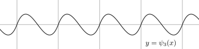
In other words (a) $\psi_{2n+1}(0) = 0$, (b) $(-1)^{n+1}\psi_{2n+1}(x)$ is positive in $[0,1/2)$, and (c) $\psi_{2n+1}(1-x) = -\psi_{2n+1}(x)$. Furthermore $$ { |\psi_{2n+1}(x)| \over (2n+1)! } \le { 2 \over (2\pi)^{2n} } \, , $$ which implies that $$ \big| R_{2n+1}(f)\big| \le { 2 \over (2\pi)^{2n} } \int_{k}^{\ell} \big|f^{(2n+1)}(x)\big| \, dx \, . $$ Any attempt to prove the formula has to be careful, because in fact the series rarely converges, nor is its convergence or lack of convergence usually a problem. The formula of Euler-MacLaurin is an asymptotic formula. We'll understand what this means in a moment.
$\bullet$ Why is the formula strange? Let's look at a particular and interesting class of examples. Suppose that we want to compute an infinite sum $$ f(1) + f(2) + f(3) + \cdots + $$ in which $f(x)$ and all of its derivatives are monotonically tending to $0$ as $x \rightarrow \infty$, and we know the sum to converge. It does no harm to assume $f(x)$ to be positive, and then every $(-1)^{n}f^{(n)}(x)$ is also positive. We break the sum into two pieces depending on a choice of an arbitrary positive integer $k$: $$ \big [ f(1) + \cdots + f(k-1) \big ] + \big[ f(k) + f(k+1) + f(k+2) + \cdots \ \big ] \, . $$ It will turn out that the EM formula will give us a good estimate of the second part, and that choosing $k$ large will improve this estimate. In other words, we still have to calculate some of the original sums, but EM will allow us to accelerate the computation drastically. The EM formula tells us that for $\ell > k$ $$ f(k) + \cdots f(\ell-1) = \int_{k}^{\ell} f(x) \, dx - { f(\ell) - f(k) \over 2 } + \left[ \sum_{m=1}^{n} { \beta_{2m}\over 2m} \cdot { f^{(2m-1)}(\ell) - f^{(2m-1)}(k) \kern6pt \over (2m-1)! } \right] + R_{2n+1}(f) \, . $$ If we let $\ell \rightarrow \infty$, we get an expression $$ f(k) + f(k+1) + \cdots = \int_{k}^{\infty} f(x) \, dx + { f(k) \over 2 } + \left[ \sum_{m=1}^{n} { \beta_{2m} \over 2m } \cdot { - f^{(2m-1)}(k) \kern6pt \over (2m-1)! } \right] + R_{2n+1}(f) $$ with $$ R_{2n+1}(f) = { 1 \over (2n+1)! } \int_{k}^{\infty} f^{(2n+1)}(x) \psi_{2n+1}(x) \, dx \, . $$ Since $f^{(2n+1)}$ is negative and monotonic, the remainder alternates in sign, which means that we have an equation $$ f(k) + f(k+1) + \cdots = \int_{k}^{\infty} f(x) \, dx + { f(k) \over 2 } + \sum_{m=1}^{\infty} (-1)^{m-1} { \gamma_{2m}\over 2m } \cdot { - f^{(2m-1)}(k) \over (2m-1)! } $$ which is valid in some peculiar sense. In what sense? The numbers $\gamma_{2m}$ grow rapidly, and consequently the series on the right does not generally converge. However, the left-hand side is sandwiched between any two of the partial sums on the right-hand side. (Note that all $\gamma_{2m}$ and $-f^{(2m-1)}(x)$ are positive, so signs in the sum alternate.)
Comments?
Let's look at how Euler used the formula.
Mathematicians in the early 18th century were very interested to know if one could find an explicit formula for $$ 1 + { 1 \over 4 } + { 1 \over 9 } + \cdots + { 1 \over n^{2} } + \cdots $$ At that time, the strongest evidence that this might be possible was the formula due to Leibniz: $$ { \pi \over 4 } = 1 - { 1 \over 3 } + { 1 \over 5 } - { 1 \over 7 } + \cdots $$ that follows from the expansion of the Taylor series of $\arctan x$ at $0$. Euler's first strategy was to approximate the sum numerically. This is not a trivial exercise. One can at least see that the series converges by applying the integral test, since $$ \sum_{1}^{n} { 1 \over k^{2} } = 1 + \sum_{2}^{\infty} { 1 \over k^{2} } \le 1 + \int_{1}^{n} { dx \over x^{2} } = 2 \, . $$ Therefore the sum is bounded. But if $S$ is the limit then $$ S - \sum_{1}^{n-1} { 1 \over k^{2} } = { 1 \over n^{2} } + { 1 \over (n+1)^{2} } + \cdots \ge \int_{n}^{\infty} { 1 \over x^{2} } \, dx = { 1 \over n } $$ which means that the series converges to $S$ very, very slowly. For example, if you wanted to compute $s$ to ten-decimal accuracy you would have to add roughly 10,000,000,000 terms. Not something to look forward to.
But now let's see what the EM formula tells us. We first calculate some derivatives: $$ \eqalign { f(x) &= {1 \over x^{2} } \cr f'(x) &= - { 2 \over x^{3} } \cr & \ldots \cr f^{(m)}(x) &= (-1)^{m} { (m+1)! \over x^{m+2} } \cr { -f^{(2n-1)}(x) \over (2n-1)! } &= { 2n \over x^{2n+1} } \, . \cr } $$ So that $$ { \beta_{2m} \over 2m } \cdot { -f^{(2m-1)}(x) \over (2m-1)! } = { \beta_{2m} \over x^{2m+1} } $$ and the EM formula, if we follow Euler, asserts that $$ \sum_{1}^{\infty} { 1 \over m^{2} } - \sum_{1}^{n-1} { 1 \over m^{2} } = \left({ 1 \over n }\right) \cdot \left( 1 + { 1 \over \mathstrut 2 n } + { \gamma_{2} \over n^{2} } - { \gamma_{4} \over n^{4} } + { \gamma_{6} \over n^{6} } - \cdots \ \right ) \, .$$ We can predict roughly how the series behaves. The denominators increase steadily by a factor of $k^{2}$, while the numerators increase roughly by a factor $(2n+1)(2n+2)/(4\pi^{2}) \sim n^{2}/\pi^{2}$. Thus the terms decrease until $n$ is about $N = \lfloor \pi k \rfloor$, when they start to increase. Given $k$, one reasonable strategy is therefore to calculate the sums up to $N$ and $N+1$. What we want lies between the two.
For example, if we choose $k = 5$ then we start out by calculating the finite sum $$ 1 + { 1 \over 4 } + { 1 \over 9 } + {1 \over 16 } \, . $$ The EM formula then gives us an approximation correct to $13$ decimals. That's a magical extrapolation, considering how little work is involved - about 8 non-zero terms in the EM formula are required (maing a total of twelve terms to add, as opposed to 10,000,000,000).
I'll be quick.
$\bullet$ Bernoulli polynomials. Define a sequence of polynomials $B_{n}(x)$ by first setting $B_{0}(x) = 1$ and then defining inductively polynomials $B_{n}$ fopr $n > 0$ by requiring $$ B'_{n}(x) = nB_{n-1}(x) \quad \int_{0}^{1} B_{n}(x) \, dx = 0 \, . $$ The first of these two conditions specifies $B_{n}$ up to a constant of integration, and the second fixes that. The first few of these are $$ \eqalign { B_{1}(x) &= x - 1/2 \cr B_{2}(x) &= x^2 - x + 1/6 \cr B_{3}(x) &= x^{3} - (3/2) x^{2} + (1/2)x \cr B_{4}(x) &= x^{4} - 2x^{3} + x^{2} - 1/30 \, . \cr } $$ The definition of these polynomials is certainly simple, but as even this short list suggests, they do not seem to be so simple. Immediate consequences of the definition are: (1) $B_{n}(1-x) = (-1)^{n}B_{n}(x)$; (2) $B_{n}(1) = B_{n}(0)$ for $n > 1$; (3) $B_{2n+1}(0) = B_{2n+1}(1/2) = 0$. These imply in turn (4) $B_{2n+1}(x)$ is positive in $(0,1/2)$; (5) $(-1)^{n-1}B_{n}(0)$ is positive.
How do these relate to the Euler-MacLaurin formula? I recall the formula for integration by parts: $$ \int_{0}^{1} f(x) \psi'(x) \, dx = \big( f(1) \psi(1) - f(0) \psi(0) \big) - \int_{0}^{1} f'(x) \psi(x) \, dx \, . $$ Since $B_{1}'(x) = 1$, we can therefore write $$ \int_{0}^{1} f(x) \,dx = {1 \over 2} \big(f(1) - f(0)\big) - \int_{0}^{1} f'(x) (x - 1/2) \, dx \, , $$ and the go on inductively, using $$ {1 \over n!} \int_{0}^{1} f^{(n)}(x) B_{n}(x) \, dx = {B_{n+1}(0) \over n! } \big( f^{(n)}(1) - f^{(n)}(0) \big) - { 1 \over (n+1)! } \int_{0}^{1} f^{(n+1)}(x) B_{n+1}(x) \, dx \,. $$ If we then define $\psi_{n}(x)$ to be the function of period $1$ agreeing with $B_{n}(x)$ on $[0,1]$, we recover the EM formula with $B_{n}(0)$ instead of $\beta_{n}$.
$\bullet$ Evaluating them. As we have seen, the EM series rarely converges. There is one case in which it does, however. If $f(x) = e^{xy}$ then the formula leads to the series $$ 1 = { e^{y} - 1 \over y } - {1 \over 2 } (e^{y} - 1) + \sum_{1}^{\infty} { B_{2m}(0) \over (2m)! } \cdot y^{2m-1}(e^{y} - 1 ) $$ which converges for $|y| \lt 2\pi$. This can be rewritten to show $$ { y \over e^{y} - 1 } = 1 - {y \over 2} + \sum_{1} { B_{2m}(0) \over (2m)! } \cdot y^{2m} \, . $$ Therefore $B_{2m}(0) = \beta_{2m}$.
Comments?
-
Leonhard Euler, Finding the sum of any series from a given general term.
This is a translation into English, by Jordan Bell, of the original in Latin. It is Euler's first systematic treatment of the summation formula. Many of Euler's papers have recently been translated and posted on the arXiv (twenty-five of them at the moment), with Euler assigned as the author! At least one person refers on the internet to a recent arXiv post by Euler himself. So much for current knowledge of history.
It is one of the many items available from the Euler Archive, a remarkable collection of papers by and about Euler.
-
Arthur Knoebel, Reinhard Laubenbacher, Jerry Lodder, and David Pengelley, Mathematical masterpieces, Springer-Verlag, 2007.
The last part of Chapter 1 is concerned with the Euler-MacLaurin summation formula. It contains an annotated excerpt from Euler's calculus textbook Institutiones Calculi Differentialis in which he discusses the formula. This is very valuable, but is also curiously unsatisfying. It seems a bit too narrowly focussed on Euler's treatment, without much of a modern perspective. One very odd feature is that it skips entirely over the most intriguing part of Euler's exposition, in which he derives explicit evaluations of the sums $$ 1 +{ 1 \over 2^{2n} } + { 1 \over 3^{2n} } + \cdots $$ The missing parts of Euler's exposition are contained in Pengelley's translation Excerpts on the Euler-MacLaurin summation formula, but without annotation.
Another valuable discussion of the summation formula can be found in\Pengelley's Dances between continuous and discrete.
-
Jeffrey Lagarias, Euler's constant: Euler's work and modern developments
The second section is a survey of work related to the summation formula.
-
E. Borevich and I. Shafarevich, Number theory, Academic Press, 1966.
The last chapter introduces Bernoulli polynomials in the last section of the book, and shows how they occur in early attempts to prove Fermat's Last Theorem.
-
Ronald Graham, Donald E. Knuth, and Oren Patashnik, Concrete mathematics, Addison-Wesley, 1989.
The last chapter is concerned with the Euler-MacLaurin formula.
-
The home page of the Bernoulli numbers.
Bill Casselman
University of British Columbia, Vancouver, Canada
Email Bill Casselman