Mathematics and Ecology
Rather than try to show the huge range of ways that mathematics is assisting biologists in understanding the vast landscape of modern biology, I will take a look at a rather small domain, which offers ways to look at some traditional topics from a novel point of view...
 Joseph Malkevitch
York College (CUNY)
Email Joseph Malkevitch
Introduction
Mathematics is important both because it has shown nifty "facts" (theorems) to be universally true and because of its applications. The domain of academic areas where mathematics has proved useful has increased with time. There was a period where people saw physics and mathematics as perhaps the most dramatic partnership between mathematics and one other academic discipline. However, at this point there is no academic discipline in which mathematics does not play an important role.
I have sampled several such interdisciplinary partnerships in prior columns: mathematics and chemistry and mathematics and psychology. This time, I will treat mathematics and ecology. It was thought in the past that the usefulness of mathematics in biology would be limited. This was because living organisms were too varied, too complex, too subtle for mathematical analysis. However, it has been not only stochastic (probabilistic) uses of mathematics that have garnered attention in biology, but also deterministic "models."
Biology, like mathematics, is a rich and complex subject with many parts. Thus, if one looks into "branches" of biology one finds many subdivisions of the subject, including the one beginning with the letter "A"--anatomy--to the one beginning with the letter "Z"--zoology. I was surprised that genetics and genomics were not listed but I found those on a different list of "branches," those of the "life sciences."
It is often helpful when thinking about how mathematics is used in other subjects to think about taxonomy--how one structures thinking about the way the different parts of a subject fit together. For example, no one doubts that mathematics has proved useful in the area of genetics. However time has altered the way that results in this area are organized and thought about. From the earliest of times farmers and people who raise livestock have used "mathematical thinking" to improve results--higher crop yields and livestock that fattened up more quickly. Thus, we see a mixture of traditional and emerging terms in this list:
Mathematical biology
Computational biology
Computational genomics
Bioinformatics
Ecology
Different parts of biology have drawn in different measures from the array of tools that mathematics provided to biology. Not surprisingly, typically it is a development in biology that leads to new ideas about how to use mathematics to understand the biological insight. Breakthroughs in biology have resulted in breakthroughs in using mathematical tools to help biologists. Rather than try to show the huge range of ways that mathematics is assisting biologists in understanding the vast landscape of modern biology, I will take a look at a rather small domain, which offers ways to look at some traditional topics from a novel point of view. This discussion takes place in the part of biology referred to as ecology. Ecology is concerned with the way different kinds of living things interact with each other and their environment. Once one brings one's "microscope" over this subdomain of biology, one sees that ecology, though a small part of biology, is a very varied discipline in its own terms.
Classification
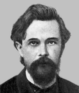
From the time of Carl Linnaeus (1707-1778), the Swedish scholar who introduced a taxonomy of living things, biologists have been concerned with the diversity of life forms on Earth and how to understand their relationships.
Portrait of Carl Linnaeus (Courtesy of Wikipedia)
Linnaeus used "strings" of words, thinking of this in mathematical terms, to help model or simplify the complex world of organisms that he saw. What Linnaeus did has had to be modernized and adapted to the ideas that have been obtained by scientists who came after him. Like all attempts to understand the "real world," the complexities of that world often challenge describing it in ways that might be as simple as we would want!
We use the hierarchical terms: domain, kingdom, phylum, class, order, family, fenus, and species. Thus, within the designation of Phylum there are many classes. However, this classification has changed with time and is not universally held. One of the reasons for change has been the way "models" are used in the sciences. Based on data, one tries to get the best models to explain the data that one can. Then, with time as new data becomes available one tries to make sure that the new data is explainable in the current model; otherwise, the model needs to change to get a better understanding of the current state of the data.
Prior to the Crick-Watson revolution in understanding genetics the classification of animals was based on various characteristics, including visual appearance. Dogs come in a vast array of sizes and kinds but for the most part zoologists agree which animals are dogs and which are not. However, in the case of some animals it was unclear which ones were "close" and which ones "far apart." The sequencing of genomes for different animals enables a new "metric," different from physical appearance, to be used to tell things that are close or far apart. So one might be tempted to group as "close" living creatures that can fly, birds, insects, and bats, but not surprisingly, insects and birds seem rather far apart when one looks at them in terms of genes. The sequencing of the genomes of different living things was part of what drove the recent adjustments to the taxonomy of living beings. If the genomes of species X and Y, viewed as closely related species in the past, were far apart there was incentive to adjust the classification system to take this into account.
Thus, Linnaeus had three "kingdoms"--animals, plants and minerals. This third kingdom was dropped because minerals (though they can "grow") are not alive. However with the advent of genome sequencing it was discovered that there was good reason to have more "kingdoms," organized somewhat differently from plants and animals. In fact, it was decided that there should be a category above kingdom, often referred to as a domain. The three domains often now used are Archaea, Bacteria, and Eukary. Archaea were a kind of microbe which seemed to be sufficiently different from other kinds of microbes to warrant special attention. Thus, in 1977, based on work of Carl Woese and George E. Fox, the traditional system of classification was modified and the "kingdoms" reorganized within the category of the three domains given above.
What is ecology?
Ecology is the branch of biology which is concerned with how organisms relate to each other and the environments in which they live. Humans share the Earth with many other life forms, as Linnaeus and his successors discovered. Wherever one lives, whether it is New York City or the Amazon, one only sees a small part of the diversity of species that the Earth has. Curiosity about these life forms is why zoos are so popular. It has also led to using scientific ideas to understand how man interacts with and uses other life forms (for food, medicine, etc.). And where there is science, there is mathematics. In ecology, as elsewhere, one uses numbers to both count and to measure.
When one makes measurements on things, say the weight of elephants in a certain region, investigators usually aim to measure the weight of all the elephants or take a sample of elephants and try to extrapolate from the sample information about the population. When populations are large, it is hard to take measurements for all of its individuals. On the other hand, when one takes a sample it is often difficult to be "sure" that the sample is representative of the population. Are the elephants in American zoos "typical" or all elephants? In getting understanding of a collection of data, there are two fundamental concepts involved. One is the notion of a measure of central tendency--a single number that captures the values of one's data set. Common measures of central tendency are the mean (the sum of the measurements divided by the number of members in the population), the median (after arranging the data in increasing order, a measurement in the middle), and the mode (a measurement which occurs most often). Not surprisingly it is hard to capture a whole population with a single number, since one data set may have nearly all the values very close to say, the mean, while another population may have the same mean as the first population but be "spread out." So it is natural in addition to a measure of central tendency for a data set to also compute a measure of "dispersion." A dispersion measure tries to indicate how far spread out the data is about the number computed for its "central tendency." A typical example is to use the mean as a measure of central tendency and the standard deviation as a measure of dispersion about the mean. Another measure of dispersion for a set of data would be the range, the difference between the largest and smallest measurements. Having thought of the range, one might invent the measure of central tendency, the "mid-range" value--the value of the range divided by two. Population means and standard deviations and sample means and standard deviations are the tools that mathematicians (statisticians) use to understand what is going on in comparing two populations. The general tools of the statistician are also the tools of the ecologist. Ecologists have invented a variety of "indices" to measure and get insight into living things.
When trying to understand species diversity, if one has two sets of "traps" (collection stations) and collects from these traps just information about the numbers of species found, one can try to sort out that there may be many species at one trap and fewer at another, but the first trap may have approximately equal numbers of each species that are found, while the other trap may have very disparate values for the species found. Thus, one trap might have 5 species where the numbers for each of these species vary from 1 to 8 while the other trap may have found 11 species but only 2 or 3 individuals for each of these. The many observational complexities of trying to comprehend biodiversity resulted in a variety of definitions to capture different aspects of biodiversity as well. The complexities show how results might vary from summer to winter and from one geographical region to another. Also, ecological studies for large mammals, birds, insects, and corals present different challenges to scientists.
Comments?
Rarefaction
One reason mathematics is powerful is that often the same mathematical tools can be used in vastly different applied settings. On the other hand, when modeling a problem, as a first approximation one might use the same tools in settings that have some similarities, but one has to be careful that the results found are truly meaningful over similar kinds of situations.
In order to give more concreteness to this matter let us imagine that an ecologist is trying to understand the diversity of the species that are in a well-defined geographic area. Abstractly, one might approach this by saying one is going to take several samples in the region involved to measure "species diversity." One first has to think through that counting tree species is easier than counting fish, birds, snakes, insects or algae. Another concern is avoiding injuring the sampled creatures. If you are trying to study the different kinds of trees in a certain area, the procedure used will be quite different from studying rodents, moths or beetles. There are interesting questions related to where you might want to take the samples, given different geographical settings. Is the "region" a lake, a river, an irregular field, or a rectangular section of a forest? While it is intriguing to contemplate the different mathematical approaches to this relatively circumscribed collection of sampling situations, my goal is to say a bit more about how some simple situations of this kind have generated mathematical ideas which have grown to be useful in a range of settings.
One of the spices of life, wherever you live, whether in a large city, suburb, or rural area, is that you see living things other than other humans. In a large city you see squirrels and pigeons in the "animal" department and various flowers and trees in the "vegetable" department. In rural areas you might see deer or foxes. However, the largest reservoir of variety of life forms is found in areas that are not heavily populated by humans or have been set aside as reserves for "wildlife," in the ocean, or "underground." We tend to concentrate on life forms with our unaided eyes but there is also the tremendous variety of bacteria that exist.
When humans think of biological diversity, they often think of how many species there are. Mathematics has been used in a number of ways to get a comprehensive look into this issue. However, given that the world is a dynamic place, the issue of even counting species is not a total "triviality." Ecologists have done lots of work to try to understand the nature of the Earth's ecosystems and to understand the complex picture of life on our planet. What is the distribution of large mammals in terms of temperature zones? One might intuitively think there would be more large mammals in the tropics than in the cold regions near the poles. What can one learn from collecting data? What about the spread of trees and flowering plants as one moves from the equator towards either the North or South Poles? Is there more diversity of life in the oceans or on land? How are insects distributed across the different temperature zones?
Perhaps the simplest way to analyze species diversity is to count species. However, this is not as simple as it might appear because telling species apart is not all that easy. It may not be hard to tell a tiger from an elephant but at a given time or location it is easier to tell the presence or absence of a species if one knows what one is looking for and can tell apart the things that one actually sees! To many people lots of different kinds of beetles look alike. How do you measure how many different birds a country has since many bird species do not spend their whole lives within one country's borders? Some countries have very few lakes and rivers and so don't have many marine species.
The regions of a large country may take pride in the number of different species present in those regions (e.g. states within the United States), but what accounts for the different numbers of species may be the size of the region, its latitude (in a general way, in the Northern Hemisphere more northerly latitudes have fewer species) and the human population of the region. Leaving aside many of the subtle questions hinted at above, how does one "measure" the number of species present in a particular locale? Perhaps the simplest such measure is to count the number of species--take a census. However, we know from counting humans that the problem of counting humans, no less squirrels in NY State, is not an easy task. Not surprisingly, one turns to statistics as a tool for using partial information (samples) to get information about the populations involved. One might try to answer questions about presence or absence of species by employing collection stations.
Mathematics might be involved in where to place the collection stations for the study. Placing them close to each other might not show the full "range" of diversity of species but stations which are close to each other might help "sort out" the consistency with which species appear in a particular locale. There are other placement issues depending on the nature of what is being counted. To understand marine diversity in a lake which is approximately circular, what mixture of collection stations near the shore versus the interior of the lake should be used? At what depth in the water should stations be placed since different marine life may be present at different depths?
So for simplicity let us imagine that the non-obvious places to put two traps to look for "creatures" (fish, eels, etc.) in a lake have been chosen and installed. To get you thinking about some of the issues the following (artificial) example shows the results of setting two collection stations, one in the East (E) and one in the West (W) of a certain region and obtaining counts of animals (say, rodents) encountered and the species they belong to.
|
|
E (East) |
W (West) |
|
1 |
8 |
1 |
|
2 |
0 |
2 |
|
3 |
2 |
0 |
|
4 |
5 |
0 |
|
5 |
1 |
1 |
|
6 |
1 |
0 |
|
7 |
0 |
3 |
|
8 |
2 |
0 |
|
9 |
0 |
5 |
|
10 |
2 |
0 |
|
11 |
1 |
0 |
|
Total species |
8 |
5 |
|
Total animals |
22 |
12 |
Table 1 (Species recorded at two collection stations)
What one notices immediately is that some species don't occur at one of the two collection stations and that when there is a species that appears at both stations, it may appear at one collection station much more often than at the other collection station. One sees that there is a large difference in the "sample" numbers found in the two collection stations--one collected 10 more items than the other. While there were 11 species represented in the two collection stations, one station found 8 species and the other only 5 but that was the station that collected fewer animals.
So what concepts might we use to get insight? One might just count how many species one finds. This measure of biodiversity is known as species richness. What is the species richness of the Earth? Rather astonishingly, the estimates for the number of species on the Earth are highly variable. A recent attempt to try to pin the numbers down (1911) resulted in the following estimates:
Animal species: 7.8 million of which 953,434 have been "described."
Plant species: 300,000 with only 215,644 being "described."
Fungi species: 610,000 of which 43,271 have been "described."
Taking into account other categories, there are an estimated 8.7 million eukaryotic species on Earth. A eukaryote is an organism which has a cell structure and the cell has a nucleus, containing genetic material in the form of chromosomes. This term is used in contrast with prokaryote, where there is no distinguished nucleus. The eukaryotes include both plants and animals. The prokaryotes include the bacteria and the relatively recently discovered archea. Human ignorance even about the numbers of species we share the Earth with is astonishing!
When you ask "ecological" questions about species richness you see tremendous variation by continent, by country, and by type of species. One country may be rich in birds but not in snakes and another country may be rich in trees but not in large mammals. Looking at patterns in ecology generates many questions and insights just as in mathematics. One especially interesting issue is species richness on "islands." Of course islands come in various sizes. Australia (which when thought of as a continent also includes the island of Tasmania) is very large and can be thought of as an island, whereas Greenland is an island but not considered a continent. Australia is considered a continent but some downplay the aspect of its being an "island." Again, definitions are complex and interesting in mathematics as well as other intellectual areas. The reason islands are relatively important to ecologists is that questions about species evolution may be easier to study for a collection of species on an island than would be the case for a region where species can move to other areas for food and breeding with more ease. When climate changes occur, species on an island will perhaps react to the these changes in a different way to species that live in an area where "migration" is easier. Australia's large size and low human population size make it particularly interesting for comprehending evolutionary questions.
Returning to Table 1 above, after examining the entries it is natural to wonder whether the East or West has more "diversity." Perhaps the differences one sees is a result of the smaller sample in the West. Ecologists reacted to this issue by developing a concept known as "rarefaction." The idea would be to see what you might expect by way of diversity in a sample of a smaller size, given that you had the information in the larger sample. A large literature has been developed in conjunction with looking at the rarefaction issue.
Below appears the expression for the computation necessary when you have two samples, one larger than the other, and where S is the number of species found in the two samples. N is the number of items found in the larger sample and n is the number of items in the smaller sample. We will assume there are a total of S different species in the two samples, but some of these may not occur in the sample which is larger. If a species does not get collected in the larger sample but only in the smaller one, it will not make a contribution to the value of E(S). So again, in slightly different words, E(S) is the expected number of species that would be found in a sample of the size of the smaller collected sample, based on the information in the larger collected sample.

(*)
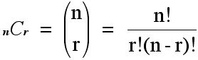
Let me remind you of some of the ideas related to the symbols that appear above. In general, given n objects, n choose r, denoted by:
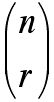 or
or 
represents the number of (non-ordered) ways that r things can be selected from n. For example, if we have 4 species, A, B, C and D, the ways that we can capture two of the species at a capture station are: A and B, A and C, A and D, B and C, B and D or C and D, for a total of 6 possibilities. Note that capturing A and D is the same as capturing D and A. The value of
nC
r can be derived from the "Fundamental Theorem of Counting." This result says that if a task A can be done in
n ways and once task A is done, task B, whatever the outcome for task A, can be done in
m ways, then task A followed by task B can be done in
nm ways, the product of
n times
m. If I have 8 shirts and 5 pairs of pants, I can appear in 40 different outfits. Using this basic idea, one can see that
nC
r has the value shown below, where
k! denotes (
k)(
k-1)...(3)(2)(1). So 5! would be equal to 5(4)(3)(2)(1).
Thus, 5C2 is 10. Intuitively, this expression will allow you to compute given, say, 6 species that it you put out a trap, what are the different numbers of ways you can catch exactly 2 of the 6 species in a trap? Thus, you can check that 6C2 = 15. Again, we are counting unordered pairs, i.e. A and D in a trap is the same outcome as a trap with D and A. Notice that nCr = nCn-r. Thus, the number of patterns of 4 species out of 6 being found in a trap is also 15. Finally, note that the number of ways that 0, 1, ..., 6 species could be found would be 26 or 64 ways.
To carry out the rarefaction for the data in Table 1 using the data from Column E, we note that there are 4 different non-zero frequencies with which species appear in the East Trap. However, in the table below we use an entry for each of these frequencies with repeats indicated, listing the rows in decreasing order of frequency.
|
Frequency |
Expected in smaller sample |
|
8 |
1 - .00 = 1.00 |
|
5 |
1 - .01 = .99 |
|
2 |
1 - .19 = .81 |
|
2 |
1 - .19 = .81 |
|
2 |
1 - .19 = .81 |
|
1 |
1 - .45 = .55 |
|
1 |
1 - .45 = .55 |
|
1 |
1 - .45 = .55 |
|
E(S) |
Total: 6.07 |
Table 2
Thus, while the E sample had 8 species presented, "adjusted" for its size it has only 6.06 species, as compared to the 5 species found in the W sample of size 12. This difference no longer seems as dramatic.
In trying to understand biodiversity we want to measure the presence or absence of species in different locales. When there is interest in avoiding species disappearing or going extinct, ecologists are not only concerned with species richness but also that the species that they see are "abundant." Ecologists invented the concept of evenness for the purpose of trying to measure this kind of distinction. The basic idea might be that one locale might have a few species but these species are present in equal numbers while another locale might have many species but more erratic numbers of the species present.
It is interesting and remarkable that there are so many different conceptual frameworks for finding measures of biodiversity, indices such as the Simpson Index, the Shannon Index, Rényi Index, and many others. Some of these indices use information-theoretic ideas and others more traditional approaches explored in statistics. Furthermore, some of these indices, while invented for one purpose, perhaps in ecology, have found analogues in other areas, for example, economics. Thus, in economics indices were developed to study the the size of firms in an industry or the amount of competition (concentration) in a sector of the economy. These economics indices have similar spirits to measuring species richness, evenness, and diversity in ecology. Such indices include the Herfindahl-Hirschman and Hannah-Kay indices.
Comments?
Continuous and discrete models
One of the early interesting insights into ecology using mathematics was obtained independently by the American mathematical demographer Alfred Lotka (1880-1949) and the Italian mathematician (Samuel) Vito Volterra (1860-1940). Lotka was born in what is today the Ukraine but spent much of his career in the US. Volterra spent some of the years after the Fascists came to power in Italy in other European countries because he lost his academic job in Rome due to the racial laws against Jews. In addition to his contribution to mathematical biology he also made important contributions to the theory of integral equations.
Vito Volterra (Courtesy of Wikipedia)
Intuitively, one might be interested in the way that two species, one of which is basically a herbivore and the other a carnivore, might interact with each other. For example, rabbits eat mostly grasses and foxes eat rabbits as well as other food. One species is a predator which survives by eating the other species. Thus, when there are no (or few) predators, the prey would tend to grow "exponentially," that is, proportional to its population size. However, the growth of the prey will be diminished as the number of interactions with predators grows. As the number of predators increases, the prey's growth would diminish, here, proportionally to the "interactions" between predator and prey.
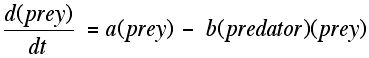

This is a system of differential equations. There are four constants that appear, and notice that you can think of the interactions between predator and prey being "independent" encounters of predator and prey. Therefore, we can "model" this by using the Fundamental Theorem of Counting (above) and take the product of the number of prey and the number of predators.
One goal of producing such models is to see if the model explains behavior that you actually see with ecological data. If you see "cycles" of increase and decline between predators and prey, does the model allow for this to be possible? From the theory point of view we can try to understand the role that the sizes of the different constants in the model have in trying to "fit" the data to the predictions of the model. Also, while there was a long history of using individual differential equations to understand the world outside of mathematics, using systems of "interlocking" differential equations and the relation of these systems to single differential equations necessitated the development of new tools in linear algebra and the theory of differential equations.
While historically differential equations were the ones that were used to construct these ecological models, you can also do this work using a difference equation or recursion. Thus, instead of looking at dy/dt, the "instantaneous" rate of change of y with respect to time, you could look at the function y(t) and study the difference y (t+1) - y(t). Here is an example of a simple difference equation: y(t+1) = 3y(t) +3. You can look for those functions which satisfy this difference equation. Difference equations are of interest both in theoretical and applied mathematics. So the famous Fibonacci numbers are governed by a difference equation while you can formulate difference equation versions of the predator-prey differential equations.
As is often the case in mathematics the development of tools to look at how predators and prey interacted in an ecological system had consequences for both "theoretical" and "applied" mathematics. Initially work of Volterra was in the context of the study of fisheries. If the prey fish are what human society values, the question comes up if one were to eliminate the predators, would the economics of fishing for the prey improve? Predator-prey situations inspired theoreticians to look at host-parasite situations. It is also possible to use similar systems of differential equations to study the properties of epidemics. What is intriguing is that different diseases require slightly different differential (or difference) equation models, so these studies have implications not only for managing breakouts of infectious disease but also for finding methods for solving different kinds of differential and difference equations.
Comments?
Markov chains
One of the most appealing mathematical models in terms of its nifty properties and wide range of applications is known as a Markov chain, named for the Russian mathematician Andrei Markov (1856-1922). Markov's son was also a distinguished mathematician.
(Andrei Markov)
As is often the case, though Markov chains have proved important in a rich collection of applications, it appears that Markov investigated them for theoretical rather than applied reasons. While in many regards Markov chains are rooted in the ideas of discrete mathematics, they also have aspects that show the fact that mathematics is a tremendously unified subject with important ideas from one part of mathematics coming into play in other parts.
Here are the basic ideas. Suppose you have a system which can be in a finite number of states, and you know the probabilities that if the system is in state i at time t, then the system will be in state j at time t+1. Furthermore, these probabilities don't change from one time step to another. These probabilities are known as transition probabilities; it might be the case that as time went on they would change but we will assume that this does not occur. As an example, which might occur in ecology, we might have a troop of baboons who travel back and forth between two regions E and A, so that in a given sequence of discretely measured time steps the members of the troop can be found in either locale E or A. We can code relevant information about the data that has been collected in the "directed graph" shown in Figure 1.
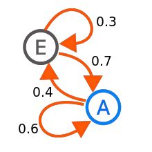
Figure 1 (Markov chain; Courtesy of Wikipedia)
The information in Figure 1 is interpreted as follows. If one is in State E, then in one time step a transition to A or back to E is possible. A similar interpretation to the line segments (directed edges) for State A can be given. The transitions follow the arrows in the diagram so for this diagram you can see that if one is in state E then one can go from E to E (stay in E) or E to A with the probabilities of these transitions indicated. The numbers on the edges in the directed graph (a mathematical tool which uses dots to represent things, and line segments with arrows joining dot X to dot Y to mean there is a relation from X to Y but not necessarily from Y to X) represent the probabilities of the different "chances" of moving between the states represented by the dots. Notice that the sum of the weights, being probabilities, on the arrows leaving a vertex add up to 1, indicating that whatever state you are currently in, in the next time step you are certain that one of the particular allowed outcomes happened. However, the sum of the numbers on the edges entering a vertex need not add to one. If we were to delete the edge from A to E with its weight of .4, we would have to adjust the weight on the arrow from A to itself, meaning that once one was in state A, one is "stuck" in state A. States where one gets stuck, once one gets there are known as absorbing states.
Another way to store the information given in Figure 1 is to use a matrix instead of a digraph. Below, for convenience we have also indicated the names of the states in addition to the numbers in the 2 x 2 matrix itself.
Figure 2 (Transition probability matrix for the Markov Chain in Figure 1)
Therefore, the entry in row A, column E means that if the system is currently in State A it will move to State E during the next time step with probability 4/10. The reason for use of matrices is that it turns out that using matrix multiplication we can determine, given probabilities that a system is in State A or State E initially, what will be the probabilities of being in State A and E after k time steps. Note that the theory here allows for the possibility that we start in A for sure, we start in E for sure or we are in state A initially with probability .97 and in State E with probability .03.
A regular Markov chain is one for which some power of the transition probability matrix has all of its entries positive. In particular this means that whatever state you might be in at a particular time, eventually you could get to any other state with positive probability. For regular Markov chains the amazing fact is that whatever is true initially, as we move through time, with higher and higher probability there is a fixed probability of being in a particular state. In algebraic terms as we raise the matrix in Figure 2 to higher and higher powers the resulting matrix approaches a matrix where all the rows are identical and have entries which are positive, between zero and one, and add to one. (In our example, this "limiting" matrix would be a 2 x 2 matrix but in general, for an n-state Markov chain, the "limiting" matrix would be n x n. Sometimes this is stated that Markov chains forget their past, that is, whatever state the system may start with initially, in the long run it will be in a particular state with a fixed probability.
We can use a bit of algebra to determine what this "limiting" collection of probabilities is for the Markov chain example involving E and A (Figure 1 and Figure 2). Let us solve for the probabilities that if we are in States E and A with probabilities e and a, then we will be in exactly these states with the same probabilities using one time step later. The equations below arise using matrix multiplication (on the left by (a, e)):
.6a + .7e = a
.4a + .3e = e
These two equations give the same information, but we also know that a + e =1 holds.
So we must solve the system:
-.4a + .7e = 0
a + e = 1
Using the methods from high school algebra we get:
a = 7/11
e = 4/11
Thus, whatever the initial situation involved you will be in state A 64 percent of the time and State E 36 percent of the time. In terms of the context of our baboon troop, the troop will be found in region A about 64 percent of the time.
I have touched on but a very small portion of ecology and the way that this subject builds on mathematical ideas. New ecological data and discoveries draw on mathematics to explain what is being learned and encourages mathematicians to build new techniques for the benefit of both mathematics and ecology.
Comments?
References
Altman, E. and J. Rhodes, Mathematical Models in Biology: An Introduction in A Biologists Guide to Mathematical Modeling in Ecology and Evolution, S. Otto and T. Day (eds.)
Britton, N., Essential Mathematical Biology, Springer Science & Business Media, 2012.
deVries, G. and T. Hillen, M. Lewis, J. Muller, B. Schoenfisch, A Course in Mathematical Biology, Vol. 12. SIAM, 2006
Edelstein-Keshet, L., Mathematical Models in Biology, Vol. 46. SIAM, 1988.
Ellner, S. and J. Guckenheimer, Dynamic Models in Biology, Princeton University Press, 2011.
Gotelli, N., A Primer of Ecology, Sinauer, 1995.
Hallam, T. and S. Levin, eds. Mathematical ecology: an introduction. Vol. 17. Springer Science & Business Media, 2012.
Hill, M. Diversity and evenness: a unifying notation and its consequences, Ecology, 54 (1973) 427-432.
Hirschman, A., The paternity of an index, The American Economic Review (1964) 761-762.
Hulbert, J., The nonconcept of species diversity: A critique and alternative parameters, Ecology 52 (1971) 577-586.
Hunter, P. and M. Gaston. Numerical index of the discriminatory ability of typing systems: an application of Simpson's index of diversity, Journal of Clinical Microbiology, 26 (1988): 2465-2466.
Jost, L., Entropy and diversity, Oikos, 113 (2006) 363-375.
Kot, M., Elements of mathematical ecology, Cambridge University Press, 2001.
Krebs, C., Ecological Methodology, (2nd ed.), Addison-Wesley, 1999.
Levin, S., Population models and community structure in heterogeneous environments, Mathematical Ecology, 1986, 295-321.
Levin, S., The problem of pattern and scale in ecology, Ecology, 73 (1992) 1943-1967.
Levin, S. and T. Hallam, and L. Gross, eds. Applied mathematical ecology. Vol. 18. Springer Science & Business Media, 2012.
MacArthur, R. and E. Wilson. The theory of island biogeography. Vol. 1. Princeton University Press, 1967.
Magurran, A. Ecological Diversity and its Measurement, Princeton University Press, Princeton, NJ, 1988.
Magurran, A., Measuring Biological Diversity, Blackwell, Oxford, 2004.
Pielou, E. Mathematical Mcology. John Wiley, 1977.
Roberts, F.. Discrete Mathematical Models, with Applications to Social, Biological, and Environmental Problems. Prentice-Hall, 1976.
Rosenzweig, M. L. 1995. Species Diversity in Space and Time. Cambridge University Press, New York, NY.
Schoener, T. and S. Boorman, Mathematical ecology and its place among the sciences, Science (1972): 389-394.
Simberloff, D., Properties of rarefaction diversity measures, American Naturalist, 106 (1972) 414-415.
Stiling, P., Ecology, Third Edition, Prentice-Hall, Upper Saddle River, 1999.
Taubes, C., Modeling Differential Equations in Biology, Prentice Hall, 2001.
------------------------------------
Special issue on Mathematical Biology:
American Mathematical Monthly, Issue 9, Volume 121, November, 2014.
Those who can access
JSTOR can find some of the papers mentioned above there. For those with access, the American Mathematical Society's
MathSciNet can be used to get additional bibliographic information and reviews of some these materials. Some of the items above can be found via the
ACM Portal, which also provides bibliographic services.
Joseph Malkevitch
York College (CUNY)
Email Joseph Malkevitch