Petals, Flowers and Circle Packings

Please note that this exposition is meant to convey a big picture so we will purposely take a few shortcuts and skip over some details and technicalities, which can be found in the references...

Introduction

The humble circle may not appear to be the most exciting candidate for further mathematical investigation. In this column, however, we will see how circle packings bring together some important ideas in geometry, topology, and analysis, and form a bridge between the discrete and continuous worlds.

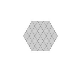
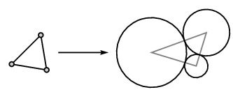
To introduce circle packings, we begin with a two-dimensional oriented surface $S$. In the example on the left below, the surface is topologically equivalent to a closed disk. We then consider a triangulation $T$ of the surface, a decompostion of the surfaces into triangles that fit together edge to edge.

 

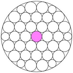
Here is a circle packing associated to this triangulation:

 

Generally speaking, a circle packing is associated to a triangulation $T$ when

 

	1. A circle is associated to each vertex of the triangulation.
	2. An edge implies a tangency between the two circles associated to its endpoints.
	3. A face implies a triple of tangencies.

To see that the circle packing above is associated to the triangulation $T$, we draw the nerve of the packing by adding a vertex at the center of each circle and edges for tangent circles.

 

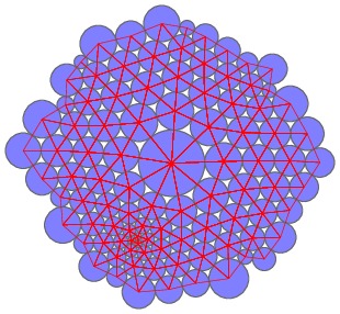
If we add triangular faces to the nerve, we find the carrier of the circle packing, which is a triangulation $T'$ of a new surface $S'$. Notice that $S'$ is topologically equivalent (homeomorphic) to the original surface $S$ and $T'$ is combinatorially equivalent to the original triangulation $T$. The carrier, therefore, provides a geometric realization of the triangulation $T$.

 

$T'$ triangulates $S'$	$T$ triangulates $S$

Thinking more generally, there is no reason to restrict ourselves to circle packings in the Euclidean plane ${\Bbb C}$; we may also look for packings in the hyperbolic plane ${\Bbb D}$ and the Riemann sphere ${\Bbb P}$. For instance, here is a packing of the same complex in the hyperbolic plane.

 

Furthermore, we may begin with a triangulation of any two-dimensional oriented surface, either with boundary or without; for the sake of simplicity, however, we will only consider simply connected surfaces here. (Remember that a surface is called simply connected if any loop on the surface may be continuously shrunk to a point.)

Please note that this exposition is meant to convey a big picture so we will purposely take a few shortcuts and skip over some details and technicalities, which can be found in the references. With that in mind, let's learn how to construct circle packings.

 

How to construct circle packings

The first questions we should ask are when do circle packings exist and how can we construct them. But before we begin thinking about these questions, let's consider a simpler problem with a similar solution.

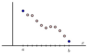
A relaxation method: Suppose we would like to find a linear function $f(x)$ on the interval $[a,b]$ having prescribed values at $a$ and $b$.

 

Of course, we know there is a unique linear function satisfying this condition. A method known as relaxation provides an algorithm to find it.

Notice that linear functions are characterized by a local condition; namely, the value of the function at a point $c$ is the average value of $f$ at two points equally spaced from $c$. That is,

$$f(c)=\frac{f(c-h)+f(c+h)}{2}.$$

 

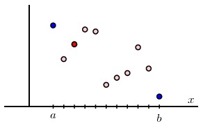
To begin our algorithm, we construct an equally spaced grid of points $x_0, x_1, \ldots, x_n$ where $x_0 = a$ and $x_n = b$ and randomly assign values to the interior points.
Starting with the leftmost point $x_1$, we replace the value at $x_1$ by the average value of its neighboring points.
We then do the same for $x_2$.
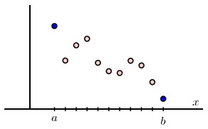
Iterating through all the interior points, we have new values:
Iterating again gives:

 

 

After 10 and 25 iterations, we have

 

Notice that each step of the algorithm disturbs the local condition we established at the previous step. Nevertheless, the values at the interior points converge to the values of the linear function we seek.

More generally, this relaxation method applies in higher dimensions to the problem of finding harmonic functions whose boundary values are prescribed.

Using the same idea, we will find a circle packing for a triangulated two-dimensional oriented surface with boundary. Let's consider the triangulation of the closed disk shown here

 

and suppose that we specify the radii of the circles associated to the boundary vertices.

 

Finding the radii: We will determine the radii of the circles associated to the interior vertices to create the circle packing

 

 

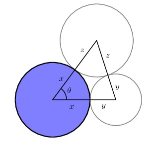
As in the relaxation method we used to find a linear function, we need an appropriate local condition determined by a circle packing. We therefore consider a single interior vertex $v$, its associated circle, and its neighbors in the packing. The neighboring circles are called petals, which together with the circle associated to $v$ form a flower. Notice that the measures of the angles meeting at this vertex add to $2\pi$. We will denote by $\theta_v$ the angle sum at $v$, the sum of the measures of the angles in all the faces meeting at $v$. As we just saw, $\theta_v = 2\pi$ for an interior vertex in a circle packing.
Notice that we may determine $\theta_v$ knowing only the radii of the circles. For instance, $\theta_v$ is the sum of angles $\theta$ obtained using the law of cosines. $ \displaystyle\theta = \arccos\frac{(x+y)^2 + (x+z)^2-(y+z)^2}{2(x+y)(x+z)}. $
Now, we begin our algorithm by randomly assigning radii to the interior circles.
Most likely, we do not have a circle packing so we need to adjust the radii of the interior circles. For example, the radius of the blue circle is too large, which our algorithm detects by computing that $\theta_v < 2\pi$.
We then compute the radius required of this interior circle so that $\theta_v=2\pi$, and we update the radius of the interior circle to this new value.

Proceeding as in our algorithm for finding the linear function, we apply this step to each of the interior vertices in turn. Of course, updating the radius of one circle may disturb an angle sum that we had previously corrected. Consequently, after one pass through all the interior points, we most likely do not have a circle packing; however, it is possible to prove that the total error in the angle sums has decreased. Therefore, we continue making passes through the interior vertices updating their radii until all the angle sums are within a desired tolerance of $2\pi$.

Finding the centers: Now that we have the radii of the interior circles, we still need to determine the centers of the circles. We choose a circle $C_0$ of radius $r_0$ and one of its petals $C_1$ of radius $r_1$. Once we choose a center for $C_0$, the center of $C_1$ must lie a distance $r_0+r_1$ away.

 

We then lay out the petals of $C_0$ one at a time beginning with $C_2$, which is tangent to $C_0$ and $C_1$.

 

Continuing in this way, we place all of $C_0$'s petals.

 

We continue this process by placing the petals of $C_1$ and so on until all the circles have been laid out.

 

It turns out that the circle packing we have found is unique up to an isometry. This is clear once we note that the radii of the interior circles are uniquely determined and all the centers determined once we choose the centers of $C_0$ and $C_1$.

In the previous example, the resulting circles have disjoint interiors, in which case we call the packing univalent. It is possible, however, to choose boundary radii that lead to packings that are not univalent; shown below are two packings of the same triangulation with the one on the left univalent and the one on the right not. This possibility must be dealt with, but in this article, we will always be meeting univalent circle packings.

 

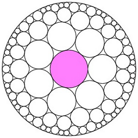
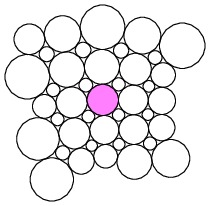
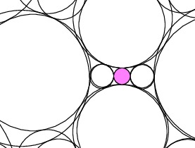
In our discussion, we constructed a circle packing by requiring $\theta_v = 2\pi$ at each of the interior vertices. Interesting examples may be found and phenomena revealed by requiring that $\theta_v = 2\pi n$ for some $n>1$ at some of the interior vertices. The two packings below have the same boundary radii; however, we require the vertex associated to the shaded circle satisfy $\theta_v=2\pi$ on the left and $\theta_v=4\pi$ on the right. This causes the petal in that flower to wrap around the central circle more than once, leading to a branching phenomenon that we will not investigate here.

 

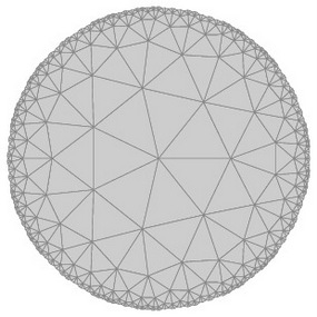
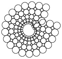
More generally, we may also create circle packings in the hyperbolic plane where the boundary circles have infinite radius; we call this the maximal packing of the triangulation $T$ and denote it ${\cal P}_T$. For example, here is such a packing of the triangulation we were just working with. This is, in some sense, a canonical packing of the surface.

 

Comments?

The Discrete Uniformization Theorem

Now that we can construct circle packings of surfaces with boundary, let's turn to triangulations of a topological open disk. We will see that there are two possible behaviors.

The parabolic case: Consider a triangulation $T$ of the plane ${\Bbb C}$ in which each vertex has six neighbors.

 

In this case, we will consider a collection of nested subtriangulations $T_k$, each of which triangulates a surface with boundary and whose union is the surface $S$.

For instance, here is such a collection for the triangulation above:

 

$T_1$		$T_2$
$T_3$		$T_4$

Since these surfaces have boundaries, our previous discussion applies. Choosing a vertex $v_0$ in $T_1$ and a neighbor $v_1$, find the maximal circle packing $P_k$ in the hyperbolic plane for each $T_k$. Lay out the circles so that $C_0$, the circle associated to $v_0$, is centered at the origin and $C_1$, the circle associated to $v_1$, is oriented along, say, the horizontal axis. In the figures below, we have highlighted the circle $C_0$.

 

$P_1$		$P_2$
$P_3$		$P_4$

Notice that the radius of $C_0$ approaches zero as $k$ goes to infinity. In fact, it appears that the radii of all the circles approaches zero.

Let us uniformly scale the circles in each packing so that the radius of $C_0$ is the same in each packing. Superimposing these packings on top of one another,

 

we see that the packings will converge to the usual hexagonal penny packing in the plane. This is the maximal packing ${\cal P}_T$ of the hexagonal triangulation in the plane ${\Bbb C}$.

 

This example illustrates a general phenomenon: whenever the radius of $C_0$ approaches zero as $k$ goes to infinity, we can in this way create a packing ${\cal P}_T$ that fills the entire plane ${\Bbb C}$. In this case, we say that $T$ is a parabolic triangulation.

The hyperbolic case: By comparison, consider an open disk triangulated so that every vertex has seven neighbors:

 

We choose a nested collection of triangulations

 

$T_1$		$T_2$
$T_3$		$T_4$

and find their circle packings in the hyperbolic plane.

 

$P_1$		$P_2$
$P_3$		$P_4$

In this case, we find that the radii of the circles $C_0$ seem to converge to a positive value, and indeed the packings seem to converge to a packing ${\cal P}_T$ that we call maximal.

This illustrates a phenomenon complementary to the parabolic case. Whenever the radii of the circles $C_0$ converge to a positive value, the circle packings converge to a maximal packing in the hyperbolic plane ${\Bbb D}$. We call such a triangulation hyperbolic.

The Discrete Uniformization Theorem: These examples illustrate the fact that we may classify a triangulation of an open disk as either parabolic, in which case its maximal packing fills the Euclidean plane ${\Bbb C}$, or hyperbolic, in which case its maximal packing fills the hyperbolic plane ${\Bbb D}$.

We have not discussed packings that arise from triangulations of the two-dimensional sphere. However, it is relatively easy to see that such a triangulation produces a packing ${\cal P}_T$ that fills the Riemann sphere ${\Bbb P}$. This leads to

 

The Discrete Uniformization Theorem: A triangulation $T$ of a simply connected surface without boundary admits a packing ${\cal P}_T$ of $T$ that fills either the Euclidean plane ${\Bbb C}$, the hyperbolic plane ${\Bbb D}$, or the Riemann sphere ${\Bbb P}$.

This theorem about circle packings is an analogue of the Uniformization Theorem for Riemann surfaces:

 

The Uniformization Theorem: A simply connected Riemann surface is conformally equivalent to either the Euclidean plane $\Bbb C$, the hyperbolic plane $\Bbb D$, or the Riemann sphere $\Bbb D$.

Comments?

Discrete analytic functions

If a complex function $f$ is analytic at a point $z_0$, then $f$ is approximately linear near $z_0$:

$$f(z_0+z) \approx f(z_0) + f'(z_0)(z-z_0)$$

or

$$ \Delta f \approx f'(z_0)\Delta z.$$

Given a complex number $m$, multiplying $z$ by $m$ has a simple geometric interpretation: $mz$ is obtained by stretching $z$ by a factor of the modulus $|m|$ and rotating $z$ by the argument of $m$. This means that the function $z\mapsto mz$ stretches and rotates the complex plane.

Analytic functions are locally represented by multiplication by the derivative $f'(z_0)$; on a small scale near $z_0$, therefore, the function $f$ stretches and rotates the plane.

For instance, consider the function $f(z)=z^2$. Shown below is a grid in the $z$-plane and its image in the $w=z^2$-plane. On this scale, the grid is bent and twisted.

 

However, if we look on a small scale near a point, we see that $f$ is simply stretching and rotating the grid. In particular, this implies that an analytic function carries small circles into small circles.

 

Let's now revisit the triangulation we considered earlier

 

and two distinct circle packings given by two sets of boundary radii.

 

Since both are packings of the same triangulation, there is a one-to-one correspondence between the circles in one packing and the circles in the other, as indicated by color. This sets up a function between circle packings that may be extended to their underlying carriers.

Since this function carries circles into circles, we may consider it to be a discrete analogue of an analytic function. In fact, such functions are called discrete analytic functions, and they behave in ways that are remarkably similar to analytic functions.

To illustrate, we can use such functions to construct analytic maps. For instance, the Riemann mapping theorem asserts that

 

If $S$ is a simply connnected, open, proper subset of the plane, then there is an invertible analytic function $f:S\to {\Bbb D}$ whose inverse is also analytic.

This is a remarkable theorem serving as a gateway to a deep understanding of two-dimensional Riemann surfaces. More simply, however, it implies the non-trivial fact that any two such subsets of the plane are homeomorphic.

Circle packings and discrete analytic functions provide a means of constructing the function $f$.

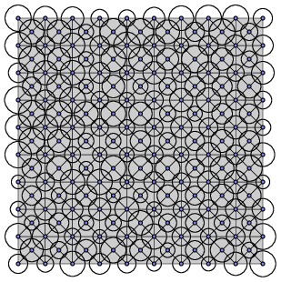
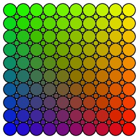
To begin, consider a bounded, simply connected open region $S$ as shown below. Choose a number $r>0$ and construct a hexagonal penny packing in the plane in which each circle has radius $r$.

 

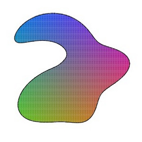
Now remove the circles whose centers lie outside $S$ to obtain a circle packing $P_r$.

 

The carrier of $P_r$ is a triangulation $T_r$ of a surface with boundary. Denote one of the circles in $P_r$ by $C_0$ and choose a point $p$ inside $C_0$. Let $C_1$ be a petal, say, to the right of $C_0$ in $P_r$. We will call $Q_r$ the maximal packing of $T_r$ in the disk ${\Bbb D}$ where the center of the circle corresponding to $C_0$ is at the origin and the center of $C_1$ is along the horizontal axis.

 

This defines a discrete analytic function $f_r:P_r\to Q_r$. We may repeat this process with a sequence $r_n$ where $r_n\to 0$.

 

$r = 0.2$
	$\stackrel{f_{0.2}}{\longrightarrow}$
$r = 0.1$
	$\stackrel{f_{0.1}}{\longrightarrow}$
$r = 0.05$
	$\stackrel{f_{0.05}}{\longrightarrow}$
$r = 0.025$
	$\stackrel{f_{0.025}}{\longrightarrow}$

Guided by the observations that discrete analytic functions carry circles into circles and that the circles in $P_r$ and $Q_r$ become increasing small, it is reasonable to expect that the discrete analytic functions $f_r:P_r\to Q_r$ approximate the analytic function $f:S\to {\Bbb D}$ described by the Riemann mapping theorem. In fact, this is the content of the Rodin-Sullivan Theorem, which was originally conjectured by Thurston:

 

As $r\to0$, the functions $f_r$ converge to the Riemann mapping $f$ uniformly on compact subsets.

 

Summary

We have just dipped our toes into the beauty of discrete analytic functions; further investigation reveals many analogies with classical analytic functions.

For instance, we saw earlier that a parabolic triangulation cannot be packed into the disk ${\Bbb D}$. This may remind you of the classical Liouville theorem. Remembering that an entire function is an analytic function defined on all of the complex plane, the Liouville theorem states

 

Liouville Theorem: There are no bounded entire functions that are not constant.

By analogy, consider a parabolic triangulation $T$ with maximal packing ${\cal P}_T$. We say that a discrete analytic function $f:{\cal P}_T\to P$ is entire if $P$ is a packing in ${\Bbb C}$, the Euclidean plane. The discrete Liouville Theorem states

 

Discrete Liouville Theorem: There are no bounded discrete entire functions.

The classical Little Picard Theorem stretches the Liouville theorem a bit further:

 

Little Picard Theorem: The image of an entire function $f:{\Bbb C}\to{\Bbb C}$ misses at most one point of the plane ${\Bbb C}$.

There is also a discrete analogue that holds providing we assume, at least for now, that the parabolic triangulation $T$ is the hexagonal triangulation $H$ of the plane.

 

Discrete Picard Theorem: A discrete entire function $f:{\cal P}_H\to P$ misses at most one point of the plane ${\Bbb C}$.

The existence of circle packings on the sphere was first proven by Koebe in 1936 and then independently by Andreev and Thurston. In fact, Thurston's use of circle packings in his work on geometric 3-manifolds is responsible for the serious attention circle packings have received recently.

Besides their intrinsic mathematical interest, circle packings have found practical use in a wide variety of applications, including "brain flattening," a process for creating flat maps of the highly convoluted surface of the three-dimensional brain.

The results described in this article are just the tip of the iceberg. While there are connections between circle packings and a rich strain of mathematical thought, one of the real pleasures for me has been implementing the algorithm to construct circle packings and running lots of examples through it. This kind of experimentation creates an almost tactile understanding of packings, which in turn leads to a deeper understanding of classical analytic functions.

Comments?

References

 

• Kenneth Stephenson. Introduction to Circle Packing. Cambridge University Press. 2005.

  As the title suggests, this book is a good place to start learning about circle packings and includes an extensive bibliography.

• Kenneth Stephenson. Circle Pack, free software for circle packing.

  I wrote my own programs to create the images in this article, but CirclePack is much more powerful and stable. I modified one of the complexes included with CirclePack and used it to create some of the images.

• William Thurston. The Geometry and Topology of 3-Manifolds. Available at http://library.msri.org/books/gt3m/.

  Thurston's seminal notes outlining, among other things, his Geometrization Conjecture for 3-manifolds. These notes first appeared in mimeographed form distributed by Princeton University. The first several chapters have been edited by Silvio Levy and have subsequently appeared in book form available from Princeton University Press through the link above.

• Charles Collins and Kenneth Stephenson. A Circle Packing Algorithm. Computational Geometry, 25, pp. 223-256, 2003.

  This article describes an efficient algorithm for creating circle packings.

• Tristan Needham. Visual Complex Analysis. Oxford University Press. 1997.


• Wikipedia pages on the Riemann mapping theorem and Uniformization Theorem.