Finding Holes in the Data
The central idea of this article is how homology theory may be used to detect topological features in noisy data sets. ...
Introduction
Across a wide range of disciplines, new technology enables us to collect, store, and process huge amounts of data. But how can we make sense of it? In this column, we'll look at how topological ideas are being used to understand global features of large data sets.
This may initially sound surprising. Topology deals with continuity. What can it possibly say about discrete sets of data points? Here's an example: diabetes occurs in two types, juvenile and adult onset. If we collect data from diabetes patients, we should expect the data to reveal the presence of these two types. We can hope that the data will coalesce into two distinct groups, which may be characterized, in some sense, as two connected components.
There is another way in which topology may be seen as a natural tool for studying data. In, say, medical studies, a large number of measurements---blood pressure, cholesterol, age, etc---may be recorded for each subject and interpreted as a vector in a large dimensional Euclidean space. However, there is not a natural way to measure the distance between the resulting data points.
For instance, with only two measurements, such as age and cholesterol ratio, we have a vector in $(a,c) \in {\mathbb R}^2$. The usual Euclidean metric $$ \sqrt{(a_1-a_2)^2 + (c_1-c_2)^2} $$ does not necessarily give an appropriate measurement of closeness since the scale of the two measurements differ by an order of magnitude. Topology provides a notion of closeness without relying on a specific measurement of distance.
Furthermore, topological thinking can reveal the large-scale structure of a data set and provide a language for describing it. More specifically, we'll see how homology theory may be used to describe the global structure of a data set and "holes" that may exist in it.
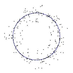
For example, suppose we perform an experiment in which we sample points on a circle and obtain the noisy data shown.
How can we detect the structure of the circle? In a typical experiment, the data set may lie in a high-dimensional space making it difficult to visualize. The central idea of this article is how homology theory may be used to detect topological features in noisy data sets. We'll get started with an informal introduction to homology theory.
Understanding homology
Intuitively, we consider two point sets to be topologically equivalent if one may be continuously deformed into the other. For instance, the sets $R$ and $S$ shown below are topologically equivalent. The corners on the boundary of $S$ are not important since they may be smoothed out with a continuous deformation.
 |
 |
| $R$ |
$S$ |
However, the sets $R$ and $T$, shown below, are not equivalent. First, any two points in $R$ may be joined with a continuous path that stays inside $R$; that's certainly not the case in $T$ in which the points are grouped into two components. Second, $R$ has two "holes" in it whereas neither component of $T$ does.
|
 |
| $R$ |
$T$ |
Homology is a powerful tool for making observations like this precise and without needing to visualize the sets we're considering. For a point set $X$, we will define, for every integer $k\geq 0$, a vector space $H_k(X)$, called the $k^{th}$ homology space. The dimensions of these spaces are called the Betti numbers of $X$ and denoted $\beta_k(X) = \dim H_k(X)$. As we'll see, the $k^{th}$ Betti number will measure the number of $k$-dimensional holes of $X$.
For instance, for the sets above, $\beta_1(R) = 2$ since there are two holes in $R$. The $0^{th}$ Betti number will measure the number of connected components so $\beta_0(R) = 1$ and $\beta_0(T) = 2$.
To make this more precise, there are many ways to define and compute homology groups. For the purposes of this discussion, we will use simplicial homology since it is intuitively appealing and will reduce our computations to a problem in finite-dimensional linear algebra.
To compute the simplicial homology of a set, we will assume that we have a triangulation of the set; that is, we assume that the set has been decomposed into a number of simplices as described below. To illustrate, here is a triangulation of our set $R$.
|
 |
| $R$ |
A triangulation of $R$ |
A $k$-simplex is a set topologically equivalent to the set in ${\mathbb R}^{k+1}$ where $$ x_0+x_1+\ldots+x_k = 1 $$ and $x_0,x_1,\ldots,x_k \geq 0.$
For instance, a $0$-simplex is a point, a $1$-simplex is a line segment, a $2$-simplex a triangle, and so forth.
 |
 |
 |
| 0-simplex |
1-simplex |
2-simplex |
Notice that the boundary of a 1-simplex consists of two 0-simplices, and the boundary of a 2-simplex consists of three 1-simplices. In general, the boundary of a $k$-simplex consists of $k+1$ simplices of dimension $k-1$.
More specifically, working in ${\mathbb R}^{k+1}$, we define $$ \begin{align} e_0=&~(1,0,0,\ldots,0) \\ e_1=&~(0,1,0,\ldots,0) \\ &\vdots \\ e_k=&~(0,0,0,\ldots,1) \end{align} $$ so that the vertices of the $k$-dimensional simplex are $[e_0,e_1,\ldots,e_k]$. The boundary of this simplex consists of $k-1$-dimensional simplices whose vertex sets are $$ \begin{align} [e_1,e_2,&\ldots,e_k] \\ [e_0,e_2,&\ldots,e_k] \\ \vdots \\ [e_0,e_1,&\ldots,e_{k-1}]. \\ \end{align} $$ In general, a $k-1$-simplex on the boundary has the form $$ [e_0,e_1,\ldots,\widehat{e_i},\ldots,e_k] $$ where $\widehat{e_i}$ means that this vertex is left out of the set.
Given a triangulation of a set $X$, we will consider $C_k$, the vector space generated by the $k$-simplices in the triangulation. We may define $C_k$ to be a vector space over any field (or even a module over the ring of integers), but in this article, $C_k$ will be a vector space over ${\mathbb Z}_2$. An element of $C_k$ is called a $k$-chain.
To measure, say, 1-dimensional holes, we will look for closed loops that enclose a hole. We therefore need a means of detecting closed 1-chains and when they enclose a hole.
To this end, we introduce the boundary map $$ \partial_k:C_k\to C_{k-1} $$ defined on a $k$-simplex by $$ \partial_k([e_0,e_1,\ldots,e_k)] = \sum_{i=0}^{k} (-1)^i[e_0,e_1,\ldots,\widehat{e_i},\ldots,e_k]. $$
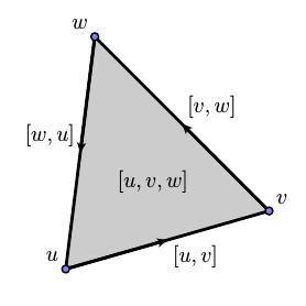
To get an intuitive sense of what this means, consider a 1-simplex, or edge, $[u,v]$ with vertices $u$ and $v$. We interpret the element $[u,v]\in C_1$ as a directed edge from $u$ to $v$ and $-[u,v]$ as the same edge directed from $v$ to $u$.
Now consider a triangular 2-simplex with vertices $[u,v,w]$ so that $$ \partial_2([u,v,w]) = [v,w] - [u,w] + [u,v]. $$ Interpreting the 1-simplices as directed edges, we see the intuitive meaning of $\partial_2$ as producing the sequence of directed edges forming the boundary of a 2-simplex.
We may now introduce two important subspaces in $C_k$:
- A $k$-boundary $b$ is a $k$-chain such that $b=\partial_{k+1}(c)$ for some $k+1$-chain $c$. In other words, a $k$-boundary is in the image of $\partial_{k+1}$, and the set of all $k$-boundaries forms a subspace $B_k = \text{Im}~\partial_{k+1}$.
 |
 |
| $[v]-[u]$ is a $0$-boundary |
The blue 1-chain is a $1$-boundary |
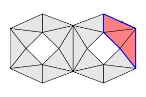
- A $k$-cycle $z$ is a $k$-chain whose boundary is zero: $\partial_k(z)=0$. The $k$-cycles also form a subspace $Z_k = \ker\partial_k$. Shown below are two $1$-cycles.
Notice that one of the cycles above is also a boundary. In fact, every boundary is a cycle. A straightforward computation shows that $\partial_k\circ\partial_{k+1} = 0$. Therefore, if $b$ is a $k$-boundary such that $b=\partial_{k+1}(c)$, then $$ \partial_k(b) = \partial_k(\partial_{k+1}(c)) = 0. $$ In other words, every $k$-boundary is also a $k$-cycle so that $B_k\subset Z_k.$
We therefore define the $k^{th}$ homology $H_k(X)$ as the quotient vector space $$ H_k(x) = Z_k/B_k. $$
In other words, $H_k(X)$ is generated by the $k$-cycles in $X$ with the added requirement that we consider two $k$-cycles equivalent if they differ by a $k$-boundary. For instance, the two 1-cycles below
are equivalent as they differ by the boundary of this 2-chain:
Applying this thinking to our example, we that any two $0$-simplices are equivalent in $H_0(R)$, as shown below. Therefore, $H_0(R)$ is a one-dimensional vector space so that $\beta_0(R) = 1$.
It is not hard to see that the 1-cycles shown below form a basis for $H_1(R)$ and therefore $\beta_1(R) = 2$.
While this seems clear intuitively, computing homology and Betti numbers can be automated. Since there are a finite number of simplices, at least in this example, the boundary maps $\partial_k:C_k\to C_{k-1}$ are linear maps between finite-dimensional vector spaces. Computing homology is then a linear-algebraic problem in which we compute the kernels and images of these maps. Moreover, if we work over the field ${\mathbb Z}_2$, the arithmetic can be performed using bit operations, which can significantly speed up the computations.
Finally, we should note that though we have defined $H_k(X)$ in terms of a triangulation of $X$, it turns out that any other triangulation produces isomorphic homology vector spaces. In other words, the homology measures intrinsic properties of $X$ rather than the triangulation.
Comments?
Persistent homology
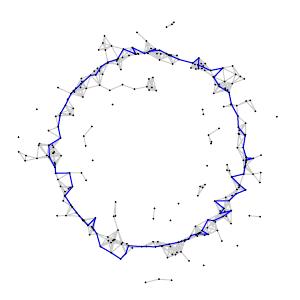
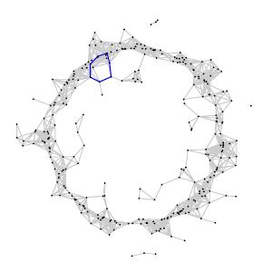
Let's return to the problem we introduced earlier. Suppose we experimentally sample points from the circle and obtain the data set shown below.
How can we apply homological thinking to discover the topological structure in the data? More specifically, can we use the data to find the one-dimensional hole in the circle?
First, we need to use the data to construct a triangulation to model the underlying circle. In doing so, we will group points that are relatively close to one another. Of course, this is precisely the problem we discussed in the introduction: in many cases, there is not a natural way to measure the distance between data points, and there often is no clear threshold for declaring points to be close.
To address the inherent ambiguity in deciding when points are close, we introduce a parameter $\epsilon\gt0$, providing a threshold to determine when two data points are to be considered close, and then allow $\epsilon$ to vary. Significant features in the data should persist across a wide range of $\epsilon$.
With a choice of $\epsilon\gt0$, we will construct a triangulation $X_\epsilon$ whose $0$-simplices are the data points themselves. Given data points $v$ and $w$, we declare $[v,w]$ to be a 1-simplex if the distance between $v$ and $w$, $d(v,w) \leq \epsilon$. Finally, $[v_0,v_1,\ldots,v_k]$ forms a $k$-simplex if $d(v_i,v_j) \leq \epsilon$ for each pair of points $v_i$ and $v_j$. The triangulation $X_\epsilon$ constructed in this way is known as a Viteoris-Rips complex.
To provide a scale, suppose that our circle has radius 1. Shown below is the set of $1$-simplices of $X_{0.2}$ on the left, and the set of $2$-simplices on the right.
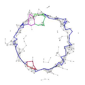
Now that we have a triangulation, we may compute the homology $H_k(X_\epsilon)$. For instance, when $\epsilon=0.2$, we find $$ \begin{align*} \beta_0(X_{0.2}) & = 7 \\ \beta_1(X_{0.2}) & = 4 \\ \end{align*} $$ A basis consisting of four $1$-cycles for $H_1(X_{0.2})$ is shown below. The seven connected components, reflecting that fact that $\beta_0(X_{0.2}) = 7$, are also clearly seen.
Now that we may compute homology $H_k(X_\epsilon)$ for every $\epsilon$, we observe that there is a natural way to compare the homology computed with different values of $\epsilon$. More specifically, if $\epsilon_1\lt\epsilon_2$, there is a natural linear map $$ H_k(X_{\epsilon_1})\to H_k(X_{\epsilon_2}). $$
To see this, remember that if $[v_0,v_1,\ldots,v_k]$ is a $k$-simplex in $X_{\epsilon_1}$, then the distance between any two vertices is less than $\epsilon_1$. Therefore, these distances are also less than $\epsilon_2\gt\epsilon_1$, which means that $[v_0,v_1,\ldots,v_k]$ is a $k$-simplex in $X_{\epsilon_2}$. This gives a natural inclusion of $k$-chains $$ C_k(X_{\epsilon_1}) \to C_k(X_{\epsilon_2}), $$ which leads to the map $H_k(X_{\epsilon_1}) \to H_k(X_{\epsilon_2})$.
Thinking more intuitively, a $k$-cycle $z$ representing an element of $H_k(X_{\epsilon_1})$ is still a $k$-cycle in $X_{\epsilon_2}$ defining an element in $H_k(X_{\epsilon_2})$. For instance, the element in $H_1(X_{0.16})$, shown on the left, persists as an element in $H_1(X_{0.22})$, shown on the right.

Imagine that we begin with a small value of $\epsilon$, which we steadily increase. A $1$-simplex $[v,w]$ first appears in $X_\epsilon$ when $\epsilon = d(v,w)$ and persists for all larger values of $\epsilon$. Since we have a finite number of data points, the set of distances $d(v,w)$ between data points forms a discrete set ${\cal D}$ of real numbers. If there is no point in ${\cal D}$ between $\epsilon_1$ and $\epsilon_2$, then the simplical complexes $X_{\epsilon_1}$ and $X_{\epsilon_2}$ are naturally equivalent and the homology spaces $H_k(X_{\epsilon_1})$ and $H_k(X_{\epsilon_2})$ are naturally isomorphic. In other words, as $\epsilon$ increases, the homology $H_k(X_\epsilon)$ may only change at the discrete points in ${\cal D}$.
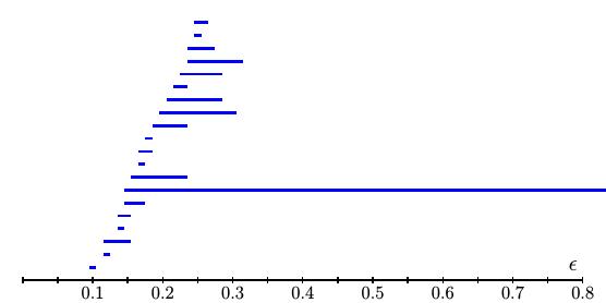
In this way, we can track elements in $H_k(X_\epsilon)$ as $\epsilon$ increases and organize their birth and death into a "barcode" as shown below.
Our basic assumption is that important features of the underlying space from which we sample will be reflected in the data over a wide range of $\epsilon$. In our example, for instance, we measure points from a circle $C$ with Betti numbers $\beta_0(C) = 1$ and $\beta_1(C) = 1$. In our barcode, we see a single generator in $H_1(X_\epsilon)$ that persists across a wide range of $\epsilon$. In fact, this generator, shown below when $\epsilon = 0.15$, reflects the generator of $H_1(C)$.
The theory that leads to homology spaces $H_k(X_\epsilon)$ and maps $H_k(X_{\epsilon_1}) \to H_k(X_{\epsilon_2})$ when $\epsilon_1 \lt \epsilon_2$ is known as persistent homology and is originally due to Edelsbrunner, Letscher, and Zomorodian.
Comments?
Persistent homology and the structure of natural images
Let's now look at how persistent homology has provided insight into the structure of images taken with a digital camera. Suppose, for instance, that our camera produces grayscale images having $n$ pixels. The grayscale intensity of each pixel may be represented by an integer $p$ such that $0\leq p \leq 255$. With each pixel's intensity forming one component, our image may be represented with a vector in ${\mathbb R}^n$.
We are interested in the subset of ${\mathbb R}^n$ corresponding to all possible images produced by our camera. Surely, it will be a large subset of ${\mathbb R}^n$ since there are a lot of images we can produce. On the other hand, the complement of this subset will also be large since choosing the grayscale intensities randomly wiill produce meaningless images.
It is hoped that an understanding of how images are distributed in ${\mathbb R}^n$ will be useful in several ways. For instance, it may be possible to design better algorithms to compress images, to clean up noisy images, and to localize objects in computer-vision applications.
Since understanding such a large space seems intractable, we will instead consider $3\times3$ arrays of pixels occurring in our images, which give rise to vectors in ${\mathbb R}^9$. For many of these arrays, the grayscale intensities will be roughly constant across the $3\times3$ array of pixels since most images, such as the one below, have large areas with little contrast.
 |
| From van Hateren's image database |
We will instead concentrate on high-contrast arrays, which carry the most important visual information in the image. To this end, Lee, Pederson, and Mumford extracted $3\times3$ arrays of pixels from a database of images taken around Groningen, Holland by van Hateren. This database consists of 4167 images, each comprised of $1532\times1020$ pixels. From each image, Lee, Pederson, and Mumford extracted a random sample of 5000 $3\times3$ pixel arrays.
They also introduced a measure of the contrast of a pixel array called the $D$-norm. Of the 5000 arrays randomly selected, they kept only the 1000 arrays with the highest $D$-norm so that they could focus on the high-contrast arrays. They then perform two operations.
- First, they subtract the average grayscale intensity from each pixel to normalize each array to have an average intensity of zero. If two arrays simply differ in brightness, they will be equal after this operation.
- Next, we normalize the vectors so that the $D$-norm of each array is one. This normalization allows us to compare the geometric structure of the contrasting pixels.
The result is a set of over 4,000,000 pixel arrays lying on a 7-dimensional sphere $S^7$ in ${\mathbb R}^8$. Lee, Pederson, and Mumford believed that the set of pixel arrays should cluster around a submanifold of $S^7$ and found some results to support this hypothesis.
Later, Carlsson, Ishkhanov, de Silva, and Zomorodian used persistent homology to study a set of similarly procured $3\times3$ pixel arrays, as we will now describe.
They began by introducing a measure of the density of the arrays. Given an array $x$, $\delta_k(x)$ is the distance between $x$ and its $k^{th}$ nearest neighbor. A small value for $\delta_k(x)$ means that the density of points near $x$ is relatively high.
Different values of $k$ give different measures of the density. When $k$ is large, $\delta_k(x)$ is determined by a larger neighborhood of $x$ and so represents a density averaged over a larger region. Smaller values of $k$ give a more refined measure of density and should therefore reveal more detailed structure.
Carlsson, Ishkhanov, de Silva, and Zomorodian first looked at arrays in the high-density portion of the data set by finding the arrays in the lowest 30th percentile of $\delta_{300}$. They then analyzed this set using persistent homology. The resulting barcode for $H_1$ showed a number of short lines and one very long one suggesting that the first Betti number $\beta_1 = 1$. In fact, a generator for this loop is the primary circle as shown below.
We interpret this as meaning that the most frequently occurring arrays are those for which the grayscale intensities are given by a linear function of the pixel position.
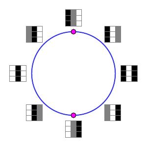
To refine this result, they next focused on the high-density arrays defined as the bottom 30th percentile of $\delta_{15}$. (Remember that for smaller values of $k$, $\delta_k$ should measure more detailed structure.) The $H_1$ barcode then implied that $\beta_1 = 5$. The primary circle shown above was still present; it was, however, joined by two secondary circles as shown below.
Notice that the arrays in the secondary circles correspond to functions of a single variable. Moving one quarter of the way around one of the circles corresponds to interpolating between a quadratic and a linear function.
While the secondary circles are disjoint, each secondary circle intersects the primary circle twice in the indicated points.
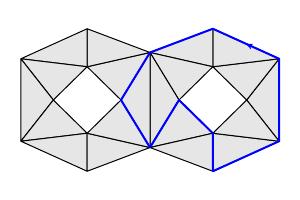
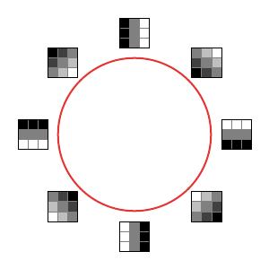
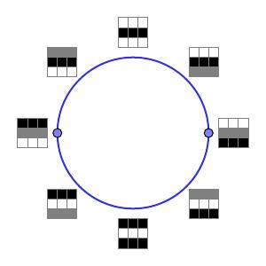
We might further ask if there is a larger 2-dimensional space in which these circles lie. Indeed, using linear and quadratic functions to describe the grayscale intensities in high-contrast arrays, Carlsson and his collaborators found in the data set a Klein bottle containing these three circles.
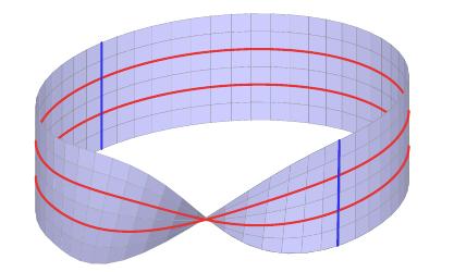
To understand this, the rectangle below will form a Klein bottle when the horizontal and vertical edges are identified as indicated by the arrows.
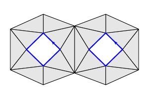
This rectangle also shows the primary (red) and secondary (blue) circles. After identifying the vertical edges with a twist, we obtain the Möbius strip below.
Finally, the Klein bottle appears when we identify points on the remaining edge so that the blue segments become circles.
One may also ask why the high-constrast arrays on the secondary circles are aligned horizontally and vertically. Surely, the camera's construction as a rectangular array of pixels plays a role. However, does nature favor such as an alignment as being more stable? To address this question, Carlsson and Ishkhanov repeated their work using $5\times5$ arrays of pixels supposing that the higher resolution would lessen any bias introduced by the camera's construction. In this new study, the primary and secondary circles appeared as before suggesting that there is some natural bias in favor of horizontally and vertically aligned arrays.
Comments?
Summary
Until fairly recently, the connections between algebraic topology and applied mathematics were rather weak, perhaps because the traditional computational strategies employed by homology theory are not well suited to applied problems. Recent work, including that described in this column, seems to indicate that this is changing. With the introduction of new software, such as Plex, a freely-available software package for computing persistent homology, we can expect to see topological methods used in a wider range of problems.
Indeed, in addition to the study of the structure of images, which we have considered here, persistent homology has been used in an analysis of the cooperation between neurons in the primary visual cortex. Carlsson's survey article describes this and a few more applications.
There are also theoretical issues that need to be addressed. For instance, when looking at our sample of $3\times3$ pixel arrays, our persistent homology calculations suggested a structure in the data. Can we be sure that this structure is not simply an artifact of the sample we have chosen? Of course, we could repeat the calculations with different samples to increase our confidence in them. However, it would be useful to have a richer statistical theory that supports drawing conclusions from these homological calculations with confidence. Again, Carlsson's survey article suggests how we might go about building a supporting theory.
References
-
Gunnar Carlsson. Topology and Data, Bulletin (New Series) of the American Mathematical Society. Volume 46, Number 2, April 2009, Pages 255-308.
Carlsson's survey article is an excellent place to start learning about persistent homology, its applications, and further questions.
-
Herbert Edelsbrunner, David Letscher, and Afra Zomorodian. Topological Persistence and Simplification, Discrete Computational Geometry, Volume 28, 4, 2002, 511-533.
-
Ann B. Lee, Kim S. Pedersen, and David Bryant Mumford. The nonlinear statistics of high-contrast patches in natural images, International Journal of Computer Vision, Volume 54, No. 1-3, August 2003, 83-103.
-
Gunnar Carlsson, Tigran Ishkhanov, Vin de Silva, and Afra Zomorodian. On the local behavior of spaces of natural images, International Journal of Computer Vision, Volume 76, 1, 2008, 1-12.
-
Hans van Hateren. Natural Image Database.
-
Afra Zomorodian and Gunnar Carlsson. Computing persistent homology, Discrete and Computational Geometry, Volume 33, 2, 2005, 247-274.
-
Vin de Silva and Gunnar Carlsson. Topological estimation using witness complexes, Eurographics Symposium on Point-Based Graphics, ETH, Zürich, Switzerland, 2004, 157-166.
-
Harlan Sexton and Mikael Vejdemo-Johansson. Javaplex software package.
Software for computing persistent homology.
 David Austin