Puzzling Over Exact Cover Problems

Posted December 2009.

This article will describe how to represent Kanoodle as an "exact cover problem" and how Donald Knuth implemented an algorithm to find solutions to exact cover problems. We'll also see how to solve Sudoku puzzles using these ideas....

David Austin
Grand Valley State University
david at merganser.math.gvsu.edu

Mail to a friend

Print this article

Introduction

For a birthday gift, one of my children recently received a puzzle called Kanoodle

that provides 12 distinctly shaped pieces:

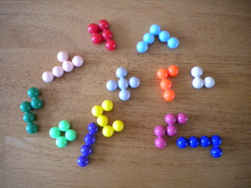
and asks the player to assemble them into a 5 by 11 rectangular grid.

Without assistance, the puzzle is extremely difficult so a booklet includes many starting configurations from which to begin.

After solving the puzzle a few times, I wondered if there was an algorithmic way for finding solutions and soon discovered that there was indeed a very interesting one. This article will describe how to represent Kanoodle as an "exact cover problem" and how Donald Knuth implemented an algorithm to find solutions to exact cover problems. We'll also see how to solve Sudoku puzzles using these ideas.

First, we will describe a generic version of the exact cover problem. Suppose we have a set S and a collection of subsets A₁, A₂, ..., A_n. We ask to find a subcollection of our subsets such that each element of S is in exactly one of the subsets.

Imagine we have the set S = {1, 2, 3, 4, 5} and subsets

A₁ = {1, 5}

A₂ = {2, 4}

A₃ = {2, 3}

A₄ = {3}

A₅ = {1, 4, 5}

Notice that the subsets A₃ = {2, 3} and A₅ = {1, 4, 5} form a solution to the exact cover problem: each element of S appears in exactly one of the sets.

In the general situation, if we have a subcollection of the sets A₁, A₂, ..., A_n, it is relatively easy to determine whether it is a solution. However, it is much more difficult to find solutions. One strategy, admittedly naive, is to consider all possible subcollections of the n sets and test each as a possible solution. The problem is that there are 2ⁿ subcollections. As we will see, the exact cover problem for Kanoodle will require us to examine a set S with 67 elements and a collection of 2222 of its subsets. The number of subcollections of the sets is the impossibly large number

2²²²² =	7738385577878121270921913291177363957675
	8053520443691507267467554511666433390225
	6211182137926950211751902449516673226756
	4728397797839387711580213688822763568480
	7079420935807010204344332535213654505000
	0110534739684220468927252571854522863758
	5111967234385629106091901532146690670721
	0178962154217210542515113476510755470378
	0036162346002513302884046411618787327146
	5491686973010799180477725197727867593234
	5632338616017848339510720332157704828285
	1869205647641463310698242417312882919566
	5264713264067983600100179414810240875191
	9075087446624702169205467746275821767903
	1488509940948129354330970633083278012074
	1650380339400461458446294783311131757068
	58291419937603163400966242304

Notice that, in this naive approach, the amount of work required grows exponentially with the number of subsets n. In fact, there is no known algorithm for finding all solutions to any exact cover problem that finishes in an amount of time bounded by a power of n. Practically speaking, this means there is no feasible algorithm for solving the exact cover problem in general. In fact, the exact cover problem is one of the NP-complete problems, a collection of problems of great interest in the theory of computation.

While there is no known algorithm that is guaranteed to find solutions to the general problem in a reasonable amount of time, we will describe an algorithm to find solutions and accept that it may not be able to produce results in our lifetimes.

Finding solutions to the exact cover problem

Let's now look at an algorithm, called "Algorithm X" by Knuth, for finding solutions to the exact cover problem. It's not particularly sophisticated; indeed Knuth refers to it as "a statement of the obvious trial-and-error approach."

Let's consider our example again, with slightly different notation. Imagine our set S is the set S = {1, 2, 3, 4, 5} and that we have subsets

A = {1, 5}

B = {2, 4}

C = {2, 3}

D = {3}

E = {1, 4, 5}

We will visualize this situation using a matrix, a rectangular array in which each column corresponds to an element of S and each row is one of our subsets. A dot in a particular cell in the matrix means that the subset corresponding to that row contains the element of S corresponding to that column.

Let's consider one of the elements of S, say, the element 1. It is contained in two subsets, A and E. Therefore, any solution to the exact cover problem must contain one, but not both, of these subsets. We will consider each of these two possibilities in turn.
Here is the basic step in the algorithm. Let's begin by looking for solutions containing the subset A. Since A contains the elements 1 and 5, any other subset containing these two elements cannot be part of a solution.
So we travel down the columns corresponding to elements 1 and 5
and eliminate any row corresponding to a subset containing 1 or 5. In this case, we eliminate subset E.
After removing these rows and columns, we are left with this simpler configuration for which we seek a solution to the exact cover problem. We now start the algorithm again from this configuration.
If we ever come to a matrix with no columns, then every element of S has been placed into a unique subset. In other words, we have found a solution. If we ever come to a matrix containing a column with no entries, then that element cannot be placed into a subset and we will not be able to find a solution with the choices that we have made so far.

Remember that we began by attempting to place the element 1 in a subset and we initially chose subset A. We also need to consider, in the same way, placing 1 into subset E and looking for solutions. In other words, from the initial configuration, we have two possible routes we must search for solutions. We will represent this with a search tree, as shown below. Each node in the tree corresponds to a particular configuration of elements and subsets. Each edge is labeled by the subset chosen to be part of the solution we seek.

Algorithm X, written more carefully, looks like:


If the matrix has no columns, we've found a solution. Stop the algorithm.
If a column has no entries, there is no solution. Stop the algorithm.
Choose a column c.
Consider each row r with an entry in c.
	Include r as part of a possible solution.
		Consider each column c' that has an entry in row r.
			Remove column c'.
			Remove each row with an entry in c'.
	Apply the algorithm to the new matrix.

We have some choice in how we implement the third step in which we choose a column c. In the example above, we have simply chosen the leftmost column at each step. However, the search tree will typically have a smaller number of nodes, which means our algorithm will finish more quickly, if we choose the column c that has the smallest number of entries.

While the algorithm, as written above, shows that we need to remove rows and columns from our matrix, we will also need to reinsert them later. For instance, in the example we stepped through above, we initially sought to place element 1 in the subset A, and this caused us to delete rows and columns from the matrix. However, we must also go back to consider placing 1 in the subset E. To do this, we need to restore the matrix to its original configuration, which requires us to reinsert the rows and columns we initially removed.

All told, we need to be able to perform a rather small set of operations. We need to be able to list all the entries in a row or column, and we need to be able to remove and reinsert rows and columns. This observation leads to Knuth's clever implementation, which he calls Dancing Links.

Implementing Algorithm X with Dancing Links

To implement Algorithm X, we will need to be able to remove rows and columns from our matrix, and we will need to be able to put them back in. In addition, we will be working with matrices having a large number of rows and columns and relatively few entries in each row. For instance, when we look for solutions to the Kanoodle problem, our matrix will have 2222 rows and 67 columns. Each row will have no more than 6 entries in it.

We could store this information, in the usual way, as a matrix containing 0's and 1's to indicate an element's membership in a particular set. However, Knuth describes a linked list structure that makes the removal of rows and columns, and their reinsertion, straightforward and requires less storage than simply storing the entire matrix.

We'll begin by describing a doubly-linked list, which is an ordered list of items together with a link from each item to its predecessor and successor. Notice that the list is circularly linked though our figures may not always indicate the links between the left and right elements.

For each element a in the list, L[a] will denote it predecessor, the element to the left of a, and R[a] will denote its successor to the right.

Notice that it is easy to remove an element from the list. For instance, if we want to remove element a, we simply reroute the links from a's predecessor and successor. That is, we reroute the links coming in to a.

We do this by setting:

R[L[a]] = R[a]
L[R[a]] = L[a]

Notice that there's no need to change the links out of a. In fact, this makes it very simple to reinsert a. Simply set

R[L[a]] = a
L[R[a]] = a

Now to implement Algorithm X, we store the columns of the matrix in a doubly-linked list. Remember that individual columns will disappear and reappear as we implement Algorithm X. We will therefore include a special element, which we'll call the root, at the beginning of the list so we'll have some consistent way to refer to the list of columns.

Each column will itself form a doubly-linked list consisting of all the entries in the rows of the matrix. Furthermore, each row will be represented in a doubly-linked list as well. The result for the matrix of our example is shown below. (As before, this figure does not show the links between the elements at the top and bottom or between the left and right.)

This is an ideal setup for implementing Algorithm X. Each element of the matrix is contained in two doubly-linked lists: one for the row and one for the column. An entire row may be removed by removing each element in the row from its column's list. Columns may be removed by removing the column header from the list of columns. Rows and columns are reinserted by adding them back into the appropriate doubly-linked list.

As the algorithm progresses, the links are continually being modified in a way that led Knuth to call this implementation "Dancing Links."

Viewing Kanoodle as an exact cover problem

We can apply Algorithm X to find solutions to the Kanoodle puzzle once we understand how to view the puzzle as an exact cover problem. Remember that we have the following pieces.

and an empty grid of 5 rows and 11 columns.

A solution is found when:

Every piece is used exactly once.
Every square in the grid is covered exactly once.

A solution will be determined by a placement of each piece on the board. We will therefore have one row in our matrix for each possible placement of each of the pieces, which leads to 2222 rows.

There will be 67 columns: one for each of the Kanoodle pieces and one for each cell in the 5 by 11 grid. A particular placement of a particular piece has an entry in the columns corresponding to the piece and the cells in the grid in which the piece lies.

For instance, this placement gives a row with five entries in the columns labeled by A, [4, 3], [5,3], [5,4], and [5,5]. (The cell [r, c] is in row r and column c.)

The search tree for Kanoodle is huge and there are many solutions. To help the algorithm run faster, I used the symmetry of the board to restrict the possible placements of the piece L. For instance, once we find a solution, we may reflect the board vertically, reflect horizontally, or rotate by a half-turn to obtain another solution. In this way, I assumed that the center of piece L is always in one of the following shaded positions, and I considered each of the possible placements of L separately.

I ran my version of Dancing Links for several hours in a few of these cases and generated many thousands of solutions, a few of which are shown below. However, my poor laptop would need more time if it were to find all of the solutions.

Since I had satisfied my initial urge to find an algorithmic means for generating solutions, and since I was interested in studying the search tree that Dancing Links traversed, I turned my attention to Sudoku puzzles.

Sudoku is also an exact cover problem

Many readers will be familiar with Sudoku puzzles, like the one shown here. There is a nine by nine grid of cells with nine boxes consisting of three by three grids. Initially, some of the cells contain one of nine possible symbols, usually chosen to be integers in the range 1 to 9. A solution is found when

Every cell contains exactly one of the symbols.
Every column has exactly one occurrence of each symbol.
Every row has exactly one occurrence of each symbol.
Every three by three box has exactly one occurrence of each symbol.

For instance, the solution (there is only one) to the puzzle above is

With the rules explained as above, we will set up an exact cover problem in which a row of our matrix corresponds to a possible way of filling a cell with a symbol. There will be 324 columns:

The first 81 are labeled by the 81 different cells and will be used to indicate that a symbol has been placed in a particular cell.
The next 81 are labeled by the nine rows and nine possible symbols. An entry in the column R = 3, S = 7 means that the third row contains the symbol 7.
The next 81 are labeled by the nine columns and nine possible symbols.
The final 81 are labeled by the nine boxes and nine possible symbols.

For instance, placing the symbol 5 in the first row and first column of the puzzle leads to a row in the matrix with four entries in the columns corresponding to (a) the cell in the first row and first column, (b) a 5 being placed in row 1, (c) a 5 being placed in column 1, and (d) a 5 being placed in the upper-left box.

The matrix is initially set up with one row for each cell whose symbol is given and nine rows for each of the other cells corresponding to the nine different symbols that may be placed in that cell. The puzzle above produces a matrix with 457 rows and 324 columns.

The complexity of the search tree that results from applying Algorithm X reflects how difficult the puzzle is. For instance, the puzzle above is labeled as "Easy," and the search tree in this case is the simplest possible: there is no branching. In other words, once we fill in the symbols given by the puzzle, there is, at every step, a cell whose symbol is uniquely determined. Algorithm X determines this rather quickly: we simply look for columns with a single entry.

By contrast, the following puzzle is labeled as "Evil."

Algorithm X completes the middle row before coming to a branching point: the cell shaded red may be filled in with either a 4 or 5.

If we put a 5 in that cell, the entries in 19 more cells are determined before we come to a dead end (it is impossible to place the symbol 9 in the seventh row):

However, putting a 4 in the red cell leads to a solution with no more branching:

The search tree for this puzzle looks like:

Evil, of course, wears many faces. The following puzzle has a search tree that is shown below and drawn without intermediate nodes to emphasize the branching at levels 30, 31, and 32.

References

Donald E. Knuth, Dancing Links, available as paper P159 at http://www-cs-faculty.stanford.edu/~knuth/preprints.html
Knuth's paper applies Dancing Links to the classic problem of placing pentominoes on a board with 60 cells, a problem very similar to the Kanoodle puzzle. In addition to describing the search tree for the pentominoes problem, he considers several other problems of a similar nature to which Dancing Links may be applied.
Knuth also offers his source code for Dancing Links at http://www-cs-faculty.stanford.edu/~knuth/programs.html. I wrote my own version in Python.
Solomon W. Golomb, Polyominoes, Scribner, 1965.
Wikipedia pages for exact cover problems and NP-complete problems.
J. Glenn Brookshear, Theory of Computation: Formal Languages, Automata, and Complexity, Benjamin/Cummings Publishing, 1989.
I obtained the Sudoku puzzles online from Web Sudoku.

David Austin
Grand Valley State University
david at merganser.math.gvsu.edu

Those who can access JSTOR can find some of the papers mentioned above there. For those with access, the American Mathematical Society's MathSciNet can be used to get additional bibliographic information and reviews of some these materials. Some of the items above can be accessed via the ACM Portal , which also provides bibliographic services.