Congressional Redistricting and Gerrymandering
We'll look at some measures that have been created to constrain gerrymandering...
Introduction
In the 2012 election for the U.S. House of Representatives, the Republican Party won 234 seats to the Democratic Party's 201. With a total of 435 seats, the Republicans' 33 seat majority represents a 7.5% advantage over the Democratics.
At the same time, Democratic candidates received 1,711,566 more votes than their Republican opponents. With nearly 125 million votes cast in the elections for congressional representatives, Democratic candidates received about 1.7% more votes.
Why is there such a disparity between the votes cast and the seats won? Though this is a complicated issue with several factors cited as influential, the process by which congressional districts are drawn is frequently cited as the most important.
In 34 states, congressional districts are drawn by the state legislature (seven states have only one representative so that the entire state forms a district), which can give the political party controlling the state legislature the power to draw districts that favor candidates of their own party.
Many states place limits on the legislature's power to draw congressional maps. For instance, most states require that districts be contiguous, meaning that one can walk between any two points in a district without leaving that district. Other requirements include respecting local political boundaries and the previous congressional map so that districts are reasonably stable. Before being weakened by a recent Supreme Court ruling, the Voting Rights Act also placed additional restrictions on certain states.
The term gerrymander refers to the act of dividing a state into districts that give unfair advantage to one political party. While there are many possibles ways to interpret what is meant by a "fair" division, two available strategies for gerrymandering are:
-
cracking, which splits a voting block into several districts thus diluting its voting power. For instance, before Ohio lost two representatives after the 2010 census, the city of Columbus was divided into three separate districts, which split up urban voters, who typically favor Democratic candidates.
-
packing, which concentrates an overwhelming majority of the political opposition in a single district. In essence, you give up one district in exchange for creating several districts in which your party enjoys a smaller, but safe, majority.
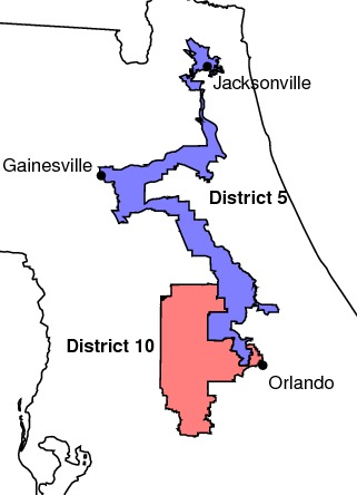
For instance, a circuit court judge recently ruled that the Florida congressional map is invalid and that Districts 5 and 10, and consequently the entire map, will have to be redrawn. In particular, District 5 appears to have been drawn with the intention of concentrating minority voters into a single district.
Similarly, voters in North Carolina have filed suit challenging their state's congressional map.

Though approximately 120 miles long, District 12 is no more than 20 miles wide and connected by a thin strip following Interstate 85.
It may seem natural to try to create an algorithm that could be used to draw congressional maps impartially. An example described by Vickrey easily shows the difficulty with this approach.
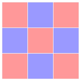
Suppose that the support for two parties in a rectangular state that is allotted four representatives is geographically dispersed as shown. Notice that a 5 to 4 majority support the red party.
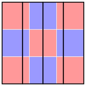
If we simply slice the state into four vertical districts, each party wins two seats.
However, if we slice the state once horizontally and once vertically, the red party wins all four seats.

Besides showing that the results can vary considerably depending on which algorithm is used, this example shows how an algorithm can lead to the very effect we are trying to avoid.
Comments?
Compactness measures
Instead, we'll look at some measures that have been created to constrain gerrymandering. Many states require congressional districts to satisfy a compactness condition. While there is no single definition of compactness, the concept attempts to identify oddly shaped regions that may be the result of gerrymandering. We'll look at a couple of different notions that have been used to measure compactness before considering a separate notion called bizarreness.
We will consider four widely-cited measures of compactness. These measures are created by comparing a district to an "ideal" simple figure, such as a rectangle or circle, with the assumption that these figures are ideal because they involve a small number of choices making them of less use for gerrymandering. A tabulation of these four measures may be found here and here.
All four measures vary from 0 to 1 with districts scoring lower judged to be less compact and hence more possibly the result of gerrymandering.
-
The first and most widely used measure, due to Polsby and Popper, relies on the isoperimetric inequality, which says this: for any simple closed curve in the plane with perimeter $P$ and bounding area $A$,then $$ 4\pi A \leq P^2 $$
and equality holds exactly when the curve is a circle. This implies that among all simple closed planar curves of the same perimeter, the circle encloses the largest area. The Polsby-Popper measure is computed as $$ \frac{4\pi A}{P^2} \leq 1 $$
The effect is to compare the area of a congressional district to the area of a circle having the same perimeter. A circular district would receive a measure of 1, while a district differing greatly from a circle would have a measure close to 0. This measure will give low scores, indicating possible gerrymandering, to districts with many indentations in the boundary or districts that are elongated in ways that stretch their boundaries without enclosing much area.
The Washington Post recently computed the Polsby-Popper measure of each of the 435 congressional districts and identified districts that stand out as possibly resulting from gerrymandering.
With a Polsby-Popper score of 0.071, Maryland's 6th District stands out. However, this appears to result from the fact that the district's boundary is partially formed by the Potomac River rather than an attempt to gain a political advantage through congressional redistricting.

The Polsby-Popper measure is easily computed using cartographic boundary files made publicly available by the U.S. Census Bureau. In those files, the districts are described as polygonal shapes with given vertices $(\lambda_i, \phi_i)$ in longitude-latitude coordinates.
-
Our second measure of compactness, due to Reock, is the ratio of the area of the district to the area of the smallest circle circumscribing the district. As in the Polsby-Popper measure, each congressional district is compared to an ideal circular district.

Though this measure may seem similar to the Polsby-Popper measure, and therefore susceptible to similar concerns about its use, Maceachren accumulated anecdotal evidence suggesting that the correlation between these two measures is only around 0.70.
-
The Schwartzberg measure of a district is the ratio of the perimeter of a district to the perimeter of a circle having the same area. Though defined similarly to the Polsby-Popper measure, these two measures are also somewhat independent of one another.

The Schwartzberg measure is quite sensitive to small variations in the boundary of the region. Remember that districts are often required to follow local political boundaries, such as townships, which could naturally cause an increase in the perimeter.
-
The Convex Hull measure is the ratio of the area of a district to that of the conex hull of the district. We may, therefore, think of this as a measurement of the convexity of the district. Convex districts, for instance, would be assigned a measure of 1, whereas districts such as the Illionois 4th District would be significantly lower and hence less compact.

Comments?
The bizareness of a district
Notice that the measures we have so far considered penalize states with irregular boundaries. In addition, they measure only the shape of the district and do not account for how the population is distributed within the district.
The last method we looked at above, the Convex Hull measure, assessed a district by measuring how convex the district is. In the same spirit, a more recent measure has been proposed by Chambers and Miller, which they call the bizarreness of a district and which may be thought of a measure of the convexity of a district.
Remember that a convex set is characterized by the fact that any two points in the set are connected by a straight line segment that is wholly contained in the set. Chambers and Miller define the bizarreness of a district to be the probability that the shortest path within the state between any two people in the district stays within the district. For instance, a convex district would have a bizarreness score of 1. Since we consider only the shortest path within the state, states with irregular boundaries are not penalized.
To be more precise, suppose that $x_i$ is the location of the $i^{th}$ person in the district. We will also define $d_S(x_i, x_j)$ to be the length of the shortest path within the state between the $i^{th}$ and $j^{th}$ person and $d_D(x_i, x_j)$ the length of the shortest path within the district. The ratio $$ \frac{d_S(x_i, x_j)}{d_D(x_i, x_j)} \leq 1, $$
and equality holds exactly when the shortest path within the state lies within the district. If there are a total of $N$ people in the district, we then define the bizarreness of the district to be $$ \frac 1{N^2}\sum_{i, j} \frac{d_S(x_i, x_j)}{d_D(x_i, x_j)}. $$
Notice that the bizarreness lies between 0 and 1 and equals 1 when the district is convex. Lower values of the bizarreness may indicate gerrymandering.
The bizarreness may be practically computed using census tracts. Suppose that a census tract within the district has population $p_\alpha$ and is centered at $x_\alpha$. Then the bizarreness may be computed by $$ \frac 1{N^2} \sum_{\alpha,\beta} \frac{d_S(x_\alpha, x_\beta)} {d_D(x_\alpha, x_\beta)} p_\alpha p_\beta. $$
Applying these measures to Maryland's 6th District, we see that
|
Measure |
Score |
|
Polsby-Popper |
0.071 |
|
Reock |
0.121 |
|
Schwartberg |
0.119 |
|
Convex Hull |
0.562 |
|
Bizarreness |
0.926 |
While the irregular shape of this district results from the state's boundary, the first four measures indicate that this district may be the result of gerrymandering. The bizarreness measure, however, indicates that it is most likely not.
If we look instead at Maryland's 3rd District, we find that all five measures indicate the possibility of gerrymandering.

|
Measure |
Score |
|
Polsby-Popper |
0.032 |
|
Reock |
0.194 |
|
Schwartberg |
0.029 |
|
Convex Hull |
0.402 |
|
Bizarreness |
0.140 |
Hodge, Marshall, and Patterson have amended Chambers and Miller's definition of bizarreness to make it somewhat easier to compute. Generally speaking, it takes some work to determine the shortest path between two points within a congressional district. Hodge and his collaborators sidestep this issue by defining a notion of semi-visibility.
Two points within a district are said to be semi-visible if the shortest path joining them only leaves the district at points on the state boundary. This is fairly straightforward to determine using the cartographic boundary files of the district and state. They then define a new measure, the boundary-adjusted convexity coefficient, to be the probability that two people in the district are semi-visible. This may again be computed using census tracts and yields results that are similar to Chambers and Miller's bizarreness measure.
Summary
As we said earlier, there is not agreement about what constitutes a fair congressional map. We have therefore been looking at an issue where reasonable people may not even agree about the nature of the problem.
Instead, we've looked at a few of the common measures that are used to indicate the possibility of gerrymandering. These have, in fact, formed part of the basis for legal arguments challenging some congressional maps.
While none of the measures is perfect, taken together they may be effective for evaluating redistricting plans. A quick Google search will reveal any number of alternative measures.
Of course, there is always what one writer has humorously called the Grofman Interocular Test: like pornography, you recognize gerrymandering when you see it.
Comments?
References
-
Christopher Chambers and Alan Miller. A Measure of Bizarreness. RepRap Home Page. Quarterly Journal of Political Science, Vol. 5, no. 1, pp. 27-44, 2010.
-
Jonathan Hodge, Emily Marshall, and Geoff Patterson. Gerrymandering and Convexity. College Mathematics Journal, vol. 41, no. 4, pp. 312-24, 2010.
-
Alan Maceachren. Compactness of Geographic Shape: Comparison and Evaluation of Measures. Geografiska Annaler, Vol. 67, no. 1, pp. 53-67, 1985.
-
William Vickrey. On the Prevention of Gerrymandering. Political Science Quarterly, Vol. 76, no. 1, pp. 105-10, 1961.
-
Edward Tufte. The Relationship between Seats and Votes in Two-Party Systems. The American Political Science Review, Vol. 67, no. 2, pp. 540-54, 1973.
-
2012 Federal Election Results.

 David Austin