A fast sweeping method for Eikonal equations

Abstract

In this paper a fast sweeping method for computing the numerical solution of Eikonal equations on a rectangular grid is presented. The method is an iterative method which uses upwind difference for discretization and uses Gauss-Seidel iterations with alternating sweeping ordering to solve the discretized system. The crucial idea is that each sweeping ordering follows a family of characteristics of the corresponding Eikonal equation in a certain direction simultaneously. The method has an optimal complexity of $O(N)$ for $N$ grid points and is extremely simple to implement in any number of dimensions. Monotonicity and stability properties of the fast sweeping algorithm are proven. Convergence and error estimates of the algorithm for computing the distance function is studied in detail. It is shown that $2^{n}$ Gauss-Seidel iterations is enough for the distance function in $n$ dimensions. An estimation of the number of iterations for general Eikonal equations is also studied. Numerical examples are used to verify the analysis.

1. Introduction

The Eikonal equation

$$\begin{equation} |\nabla u(\mathbf{x})|=f(\mathbf{x}),\nobreakspace\nobreakspace\nobreakspace\nobreakspace \mathbf{x}\in R^{n}, {\tag{1.1}} \end{equation}$$

with boundary condition, $u(\mathbf{x})=\phi (\mathbf{x}), \mathbf{x}\in \Gamma \subset R^n$, has many applications in optimal control, computer vision, geometric optics, path planing, etc. This nonlinear boundary value problem is a first order hyperbolic partial differential equation (PDE). Information propagates along characteristics from the boundary. Due to the nonlinearity, characteristics may intersect like the formation of shocks in hyperbolic conservation law. The solution is still continuous at these intersections but may not be differentiable. The existence and uniqueness of the viscosity solution are shown in 4.

There are two key ingredients for any numerical algorithm for the Eikonal equation. The first key ingredient is the derivation of a consistent and accurate discretization scheme, i.e., a numerical Hamiltonian. The numerical scheme has to follow the causality of the partial differential equation and has to deal with non-differentiability at intersections of characteristics properly. Since the problem is nonlinear, a large system of nonlinear equations has to be solved after the discretization. Hence the second key ingredient is an efficient method for solving the large nonlinear system.

There are mainly two types of approaches for solving the Eikonal equation. One approach is to transform it to a time dependent problem. For example, if we have $u(\mathbf{x})=0$, $\mathbf{x}\in \Gamma$, then $u(\mathbf{x})$ is the first arrival time at $\mathbf{x}$ for a wave front starting at $\Gamma$ with a normal velocity that is equal to $\frac{1}{f(\mathbf{x})}$. This can be solved by the level set method. In the control framework, a semi-Lagrangian scheme is obtained for Hamilton-Jacobi equations by discretizing in time the dynamic programming principle 910. However, many time steps may be needed for the convergence of the solution in the entire domain due to finite speed of propagation and CFL condition for time stability. The other approach is to treat the problem as a stationary boundary value problem and to design an efficient numerical algorithm to solve the system of nonlinear equations after discretization. For example, the fast marching method 191611 is of this type. In the fast marching method, the update of the solution follows the causality in a sequential way; i.e., the solution is updated one grid point by one grid point in the order that the solution is strictly increasing (decreasing). Hence an upwind difference scheme and a heapsort algorithm are needed. The complexity is of order $O(N\log N)$ for $N$ grid points, where the $\log N$ factor comes from the heapsort algorithm.

Here we present and analyze an iterative algorithm, called the fast sweeping method, for computing the numerical solution for the Eikonal equation on a rectangular grid in any number of space dimensions. The fast sweeping method is motivated by the work in 2 and was first used in 21 for computing the distance function. The main idea of the fast sweeping method is to use nonlinear upwind difference and Gauss-Seidel iterations with alternating sweeping ordering. In contrast to the fast marching method, the fast sweeping method follows the causality along characteristics in a parallel way; i.e., all characteristics are divided into a finite number of groups according to their directions and each Gauss-Seidel iteration with a specific sweeping ordering covers a group of characteristics simultaneously. The fast sweeping method is extremely simple to implement. The algorithm is optimal in the sense that a finite number of iterations is needed. So the complexity of the algorithm is $O(N)$ for a total of $N$ grid points. The number of iterations is independent of grid size. The accuracy is the same as any other method which solves the same system of discretized equations. The fast sweeping method has been extended to more general Hamilton-Jacobi equations 1812. Extensions to high order discretization will be studied in future reports.

The idea of alternating sweeping ordering was also used in Danielsson’s algorithm 6. The algorithm computes the distance mapping, i.e., the relative $(x,y)$ coordinate of a grid point to its closest point using an iterative procedure. Danielsson’s algorithm is based on a strict dimension by dimension discrete formulation which in general does not follow the real characteristics of the distance function in two and higher dimensions and hence results in low accuracy and twice as many iterations compared to the fast sweeping method we present here. Danielsson’s algorithm does not work for distance functions to more general data sets such as the distance to a curve or a surface. Neither does it extend to general Eikonal equations. Recently another discrete approach that uses the idea of fast sweeping method was proposed in 17. It can compute the distance function more accurately but does not apply to general Eikonal equations either. Other related methods include a dynamic programming approach and post sweeping idea in 15 and a group marching method in 13.

Here is the outline of the paper. In Section 2 we present the scheme and the motivation behind it. We then show a few monotonicity properties and a maximum change principle for the fast sweeping algorithm in Section 3. In Section 4 we prove the convergence and error estimates for the distance function. We discuss the fast sweeping method for general Eikonal equations in Section 5. In Section 6 we present numerical results to verify our analysis and we show a few applications.

2. The fast sweeping algorithm and the motivation

We present the fast sweeping method for computing the viscosity solution $u(\mathbf{x})\ge 0$ for the model problem

$$\begin{equation} \begin{array}{ll} |\nabla u(\mathbf{x})|=f(\mathbf{x}), & \mathbf{x}\in R^{n}, \\u(\mathbf{x})=0, & \mathbf{x}\in \Gamma \subset R^{n}, \end{array} {\tag{2.1}} \end{equation}$$

where $f(\mathbf{x})>0$. For simplicity the algorithm is presented in two dimensions. The extension to higher dimensions is straightforward. We use $\mathbf{x}_{i,j}$ to denote a grid point in the computational domain $\Omega$,  $h$ to denote the grid size and $u^{h}_{i,j}$ to denote the numerical solution at $\mathbf{x}_{i,j}$.

2.1. The fast sweeping algorithm

Discretization

We use the following Godunov upwind difference scheme 14 to discretize the partial differential equation at interior grid points:

$$\begin{equation} \begin{array}{l} [(u^{h}_{i,j}-u^{h}_{x\min })^{+}]^{2} + [(u^{h}_{i,j}-u^{h}_{y\min })^{+}]^{2} =f^2_{i,j}h^{2} \\\\i=2, \ldots , I-1,\nobreakspace j=2, \ldots , J-1, \end{array} {\tag{2.2}} \end{equation}$$

where $u^{h}_{x\min }=\min (u^{h}_{i-1,j},\nobreakspace u^{h}_{i+1,j}),\nobreakspace u^{h}_{y\min }=\min (u^{h}_{i,j-1}, u^{h}_{i,j+1})$ and

$$\begin{equation*} (x)^{+}=\begin{cases} x, & x>0, \\ 0, & x\le 0 . \end{cases} \end{equation*}$$

One sided difference is used at the boundary of the computational domain. For example, at a left boundary point $\mathbf{x}_{1,j}$, a one sided difference is used in the $x$ direction,

$$\begin{equation*} [(u^{h}_{1,j}-u^{h}_{2,j})^{+}]^{2} + [(u^{h}_{1,j}-u^{h}_{y\min })^{+}]^{2} =f_{1,j}^2h^{2}. \end{equation*}$$

Initialization

To enforce the boundary condition, $u(\mathbf{x})=0$ for $\mathbf{x}\in \Gamma \subset R^{n}$, assign exact values or interpolated values at grid points in or near $\Gamma$. These values are fixed in later calculations. Assign large positive values at all other grid points. These values will be updated later.

Gauss-Seidel iterations with alternating sweeping orderings

At each grid $\mathbf{x}_{i,j}$ whose value is not fixed during the initialization, compute the solution, denoted by $\overline{u}$, of (2.2) from the current values of its neighbors $u^{h}_{i\pm 1,j},u^{h}_{i,j\pm 1}$ and then update $u^{h}_{i,j}$ to be the smaller one between $\overline{u}$ and its current value; i.e., $u^{\operatorname {new}}_{i,j}=\min (u^{\operatorname {old}}_{i,j},\overline{u})$. We sweep the whole domain with four alternating orderings repeatedly:

$$\begin{equation*} \begin{array}{ll} (1)\nobreakspace i=1:I, j=1:J , & (2)\nobreakspace i=I:1, j=1:J, \\(3)\nobreakspace i=I:1, j=J:1, & (4)\nobreakspace i=1:I, j=J:1. \end{array} \end{equation*}$$

The unique solution to the equation

$$\begin{equation} [(x-a)^{+}]^{2}+[(x-b)^{+}]^{2}=f^2_{i,j} h^{2}, {\tag{2.3}} \end{equation}$$

where $a=u^h_{x\min },b=u^h_{y\min }$, is

$$\begin{equation} \overline{x}=\left\{ \begin{array}{ll} \min (a,b)+f_{i,j}h, & |a-b|\ge f_{i,j}h, \\[6.0pt] \frac{a+b+\sqrt {2f_{i,j}^2 h^{2}-(a-b)^{2}}}{2}, & |a-b|<f_{i,j}h. \end{array} \right. {\tag{2.4}} \end{equation}$$

In $n$ dimensions the unique solution $\overline{x}$ to

$$\begin{equation} [(x-a_1)^{+}]^{2}+[(x-a_2)^{+}]^{2}+\cdots +[(x-a_n)^{+}]^{2}=f_{i,j}^2 h^{2} {\tag{2.5}} \end{equation}$$

can be found in the following systematic way. First we order the $a_{k}$’s in increasing order. Without loss of generality, assume $a_1\le a_2 \le \cdots \le a_n$ and define $a_{n+1}=\infty$. There is an integer $p$, $1\le p\le n$, such that $\overline{x}$ is the unique solution that satisfies

$$\begin{equation} (x-a_1)^{2}+(x-a_2)^{2}+\cdots +(x-a_p)^{2}=f_{i,j}^2 h^{2}\nobreakspace\nobreakspace \text{and}\nobreakspace\nobreakspace a_p<\overline{x}\le a_{p+1}; {\tag{2.6}} \end{equation}$$

i.e., $\overline{x}$ is the intersection of the straight line $\mathbf{x}=\mathbf{y},\nobreakspace \mathbf{x},\mathbf{y}\in R^p$, with the sphere centered at $\mathbf{a}=(a_1,a_2, \ldots , a_p)$ of radius $f_{i,j}h$ in the first quadrant in $R^{p}$. We find $\overline{x}$ and $p$ in the following recursive way. Start with $p=1$. If $\tilde{x}=a_1+f_{i,j}h\le a_2$, then $\overline{x}=\tilde{x}$. Otherwise find the unique solution $\tilde{x}>a_2$ that satisfies

$$\begin{equation*} (x-a_1)^{2}+(x-a_2)^{2}=f_{i,j}^2h^{2}. \end{equation*}$$

If $\tilde{x}\le a_3$, then $\overline{x}=\tilde{x}$. Otherwise repeat the procedure until we find $p$ and $\overline{x}$ that satisfy (2.6).

Here are a few remarks about the algorithm:

(1)

The upwind difference scheme (2.2) is a special case of the general Godunov numerical Hamiltonian proposed in 1. The numerical Hamiltonian can be written as$$\begin{align*} &H^{h}(D_{-}^{x}u_{i,j},D_{+}^{x}u_{i,j},D_{-}^{y}u_{i,j},D_{+}^{y}u_{i,j}) \\ &\qquad =\sqrt {\max \{(D_{-}^{x}u_{i,j})^{+},(D_{+}^{x}u_{i,j})^{-}\}^{2}+ \max \{(D_{-}^{y}u_{i,j})^{+},(D_{+}^{y}u_{i,j})^{-}\}^{2}}, \end{align*}$$

where$$\begin{equation*} \displaystyle { \begin{array}{l} D_{-}^{x}u_{i,j}=\frac{u_{i,j}-u_{i-1,j}}{h},\qquad D_{+}^{x}u_{i,j}=\frac{u_{i+1,j}-u_{i,j}}{h}, \\D_{-}^{y}u_{i,j}=\frac{u_{i,j}-u_{i,j-1}}{h},\qquad D_{+}^{y}u_{i,j}=\frac{u_{i,j+1}-u_{i,j}}{h}, \end{array} } \end{equation*}$$

and $(\cdot )^{+}$ means taking the positive part and $(\cdot )^{-}$ means taking the negative part. Instead of using the upwind difference scheme (2.2), we can also use$$\begin{equation} \begin{split}[(u^{h}_{i,j}\ &-\ u^{h}_{i-1,j})^{+}] ^{2} +[(u^{h}_{i,j}-u^{h}_{i+1,j})^{+}]^{2} \\ &+\ [(u^{h}_{i,j}-u^{h}_{i,j-1})^{+}]^{2} +[(u^{h}_{i,j}-u^{h}_{i,j+1})^{+}]^{2} =f_{i,j}^2h^{2}, \\ &\qquad \qquad \qquad \qquad i=2, \ldots , I-1,\quad j=2, \ldots , J-1, \end{split} {\tag{2.7}} \end{equation}$$

which corresponds to the numerical Hamiltonian$$\begin{align*} &H^{h}(D_{-}^{x}u_{i,j},D_{+}^{x}u_{i,j},D_{-}^{y}u_{i,j},D_{+}^{y}u_{i,j}) \\ &\qquad =\sqrt {[(D_{-}^{x}u_{i,j})^{+}]^2+[(D_{+}^{x}u_{i,j})^{-}]^2+ [(D_{-}^{y}u_{i,j})^{+}]^2+[(D_{+}^{y}u_{i,j})^{-}]^2}. \end{align*}$$

Both numerical Hamiltonians are monotone. The only difference between these two formulations is at the intersections of characteristics. The second formulation may have larger truncation errors at those intersections as will be explained in Section 4.

(2)

In practice it may be desirable to restrict the computation to a neighborhood of the boundary $\Gamma$. For example, if we want to restrict the computation in the neighborhood where the first arrival time is less than $T$, i.e., $\{\mathbf{x}_{i,j}:u(\mathbf{x}_{i,j}) < T\}$, then we can use the following simple cutoff criterion: in the Gauss-Seidel iteration we update the solution at a grid point $\mathbf{x}_{i,j}$ only if at least one of its neighbors has a value smaller than $T$, i.e., if $\min (u^{h}_{x\min },u^{h}_{y\min })<T$.

(3)

The large value assigned initially should be larger than the maximum possible value of $u(\mathbf{x})$ in the computation domain. For example, let $f_{M}=\max _{\mathbf{x}\in \Omega }f(\mathbf{x})$ and let $D$ be the diameter of the computational domain $\Omega$. The initially assigned large value should be larger than $F_{M}D$.

(4)

In higher dimensions, the discretization (2.2) is easily extended dimension by dimension and there are $2^n$ different sweeping orderings in $n$ dimensions.

(5)

If we want to compute the viscosity solution $u(\mathbf{x})\le 0$ for (2.1), we modify the discretization (2.2) to$$\begin{equation} \begin{array}{l} [(u^{h}_{i,j}-u^{h}_{x\max })^{-}]^{2} + [(u^{h}_{i,j}-u^{h}_{y\max })^{-}]^{2} =f_{i,j}^2h^{2}, \\i=2, \ldots , I-1,\quad j=2, \ldots , J-1, \end{array} {\tag{2.8}} \end{equation}$$

where $u^{h}_{x\max }=\max (u^{h}_{i-1,j},\nobreakspace u^{h}_{i+1,j}),\nobreakspace u^{h}_{y\max }=\max (u^{h}_{i,j-1}, u^{h}_{i,j+1})$ and$$\begin{equation*} (x)^{-}=\begin{cases} 0, & x>0, \\ -x, & x\le 0 . \end{cases} \end{equation*}$$

In the initialization, we assign small negative values at grid points whose values are to be updated. In the Gauss-Seidel iteration, we update the value at a grid point only if the new value obtained by solving (2.8) is larger than its old value.

2.2. The motivation

In the fast sweeping algorithm the upwind difference scheme used in the discretization enforces the causality; i.e., the solution at a grid point is determined by its neighboring values that are smaller. The one sided difference scheme at the boundary enforces the propagation of information to be from inside to outside since the data set $\Gamma$ is contained in the computational domain. If all grid points can be ordered according to the causality along characteristics, one iteration of the Gauss-Seidel iteration is enough for convergence. For example, the heapsort algorithm is used in the fast marching method to sort out this order every time a grid point is updated. The key point behind Gauss-Seidel iterations with different sweeping ordering is that each sweep will follow the causality of a group of characteristics in certain directions simultaneously and all characteristics can be divided into a finite number of such groups according to their directions. The value at each grid point is always nonincreasing during the iterations due to the updating rule. Whenever a grid point obtains the minimal value it can reach, the value is the correct value and the value will not be changed in later iterations.

We use the distance function as an example to illustrate the motivation. The distance function $d(\mathbf{x})$ to a set $\Gamma$ satisfies the Eikonal equation

$$\begin{equation*} |\nabla d(\mathbf{x})|=1,\nobreakspace\nobreakspace\nobreakspace d(\mathbf{x})=0, \mathbf{x}\in \Gamma . \end{equation*}$$

All characteristics of this equation are straight lines that radiate from the set $\Gamma$. In one dimension, the upwind differencing at the interior grid point $i$ is

$$\begin{equation} [(u^{h}_{i}-\min (u^{h}_{i-1}, u^{h}_{i+1}))^{+}]^{2}=h^{2},\nobreakspace\nobreakspace\nobreakspace 2\le i \le I-1. \tag{2.9} \end{equation}$$

We use two Gauss-Seidel iterations with sweeping orderings, $i=1:I$ and $i=I:1$ successively, to solve the above system. The update of the distance value at grid $i$ simply becomes

$$\begin{equation*} u_{i}^{\operatorname {new}}=\min (\min (u_{i-1}, u_{i+1}) + h, u_i). \end{equation*}$$

Figure 2.1 shows how one sweep from left to right followed by one more sweep from right to left is enough to finish the calculation of the distance function. This follows because there are only two directions for the characteristics in one dimension, left to right or vice versa. In another word, the distance value at any grid point can be computed from either its left neighbor or right neighbor by exactly $d_{i}=\min (d_{i-1}, d_{i+1})+h$. The first sweep will cover those characteristics that go from left to right; i.e., those grid points whose values are determined by their left neighbors are computed correctly. Similarly, in the second sweep all those grid points whose values are determined by their right neighbors are computed correctly. Since we only update the current value if the newly computed value is smaller, those values that have been calculated correctly in the first sweep have achieved their minimal possible values and will not be changed in the second sweep. Convergence in two sweeps is true for arbitrary Eikonal equations in one dimension. In the special case of the distance function, it is easy to see that the fast sweeping method finds the exact distance function in two sweeps.

In higher dimensions characteristics have infinitely many directions which cannot be followed exactly by the Cartesian grid lines. Here are two important questions for the fast sweeping algorithm: (1) How many Gauss-Seidel iterations are needed? (2) What is the error estimate? The most important observation is that all directions of characteristics can be classified into a finite number of groups for distance functions. For example, in two dimensions all directions of characteristics can be classified into four groups, up-right, up-left, down-left and down-right. Information propagates along characteristics in the above four groups of directions. The four different orderings of the Gauss-Seidel iterations and the upwind differencing are meant to cover the four groups of characteristics, respectively. Figure 2.2(a) illustrates why the fast sweeping method converges after four sweeps with different orderings for the distance function to a single point. The solution $u^{h}_{i,j}$ at each grid point in the first quadrant depends on the solution at $u^{h}_{i-1,j}$ and $u^{h}_{i,j-1}$ which have already been computed and can be recursively traced all the way back to the data point in the first sweep. So we get the correct values for all grid points in the first quadrant plus the points on the positive $x$ and $y$ axes after the first sweep. For the same reason, after the second sweep the grid points in the second quadrant and on the negative $x$ axis get the correct values. Moreover, since those grid points in the first quadrant and on the positive $x$ and $y$ axes already have their minimal values and satisfy the discretized equations, these values will not change in the second sweep. Similarly, after the third sweep those grid points in the third quadrant and on the negative $y$ axis get the correct values and the computed correct values in the first and second quadrants are maintained. After four sweeps we get the correct values for all grid points that satisfy the system of equations (2.2). Figure 2.2(b) demonstrates another case which computes the distance function to a circle in two dimensions using the fast sweeping algorithm. Again, each grid point gets its correct value in one of the four sweeps.

In the case of one data point, the distance function is smooth except at the data point. For a more general data set, interactions of characteristics at their intersections can cause more than $2^{n}$ sweeps for the iteration to converge in $n$ dimensions. It is impossible to track the exact number of sweeps for the highly nonlinear discretized system in general. However, we will show that in $n$ dimensions, after $2^n$ sweeps the fast sweeping method can compute a numerical solution to the distance function that is as accurate as the numerical solution after the iteration converges. This means $2^n$ sweeps is good enough in practice for computing the distance function to an arbitrary data set. For general Eikonal equations, the characteristics are curves instead of straight lines. So more than one sweep may be needed to cover one characteristic curve. We will see that given a fixed domain and the right-hand side $f(\mathbf{x})$, the number of sweeps needed is still finite and is independent of grid size.

3. Basic properties of the fast sweeping algorithm

Here we prove a few basic monotonicity properties and a maximum change principle for the fast sweeping algorithm. The following simple fact for the solution of equation (2.5) provides the monotonicity and maximum change principle for the fast sweeping algorithm.

Lemma 3.1.

Let $\overline{x}$ be the solution to equation 2.5. We have

$$\begin{equation} 1\ge \frac{\partial \overline{x}}{\partial a_{1}}\ge \frac{\partial \overline{x}}{\partial a_{2}}\ge \cdots \ge \frac{\partial \overline{x}}{\partial a_{n}}\ge 0 {\tag{3.1}} \end{equation}$$

and

$$\begin{equation} \frac{\partial \overline{x}}{\partial a_{1}}+ \frac{\partial \overline{x}}{\partial a_{2}}+\cdots + \frac{\partial \overline{x}}{\partial a_{n}}=1. \tag{3.2} \end{equation}$$

Proof.

Differentiating equation (2.5) with respect to $a_{k}$, we get

$$\begin{equation*} \displaystyle { \frac{\partial \overline{x}}{\partial a_{k}} =\frac{(\overline{x}-a_{k})^+}{\sum _{m=1}^{n}(\overline{x}-a_{m})^+} }. \end{equation*}$$■

As a direct consequence of the lemma, we have

Proposition 3.2.

In the Gauss-Seidel iteration for the fast sweeping method, the maximum change of $u^{h}$ at any grid point is less than or equal to the maximum change of $u^{h}$ at its neighboring points.

Lemma 3.3.

The fast sweeping algorithm is monotone in the initial data.

Proof.

This is a direct consequence from Lemma 3.1; i.e., the monotonicity property of the solution to (2.5). If $u^{h}(\mathbf{x}_{i,j})\le v^{h}(\mathbf{x}_{i,j})$ at all grid points initially, then $u^{h}(\mathbf{x}_{i,j})\le v^{h}(\mathbf{x}_{i,j})$ at all grid points after any number of Gauss-Seidel iterations.

■

Lemma 3.4.

The solution of the fast sweeping algorithm is nonincreasing with each Gauss-Seidel iteration.

Proof.

This is exactly because of the way we update the solution in the Gauss-Seidel iterations described in the third step of the algorithm.

■

The following corollary shows the stability property for the fast sweeping method. We present it in two dimensions but it is true in general.

Corollary 3.5.

Let $u^{(k)}$ and $v^{(k)}$ be two numerical solutions at the $k$-th iteration of the fast sweeping algorithm. Let $\|\cdot \|_{\infty }$ be the maximum norm. We have

(1) $\|u^{(k)}-v^{(k)}\|_{\infty }\le \|u^{(k-1)}-v^{(k-1)}\|_{\infty }$,

(2) $0\le \max _{i,j}\{u_{i,j}^{(k)}-u_{i,j}^{(k+1)}\} \le \max _{i,j} \{u_{i,j}^{(k-1)}-u_{i,j}^{(k)}\}$.

Proof.

Let us assume that the first update at the $k$-th iteration is at point $\mathbf{x}_{i,j}$, $u^{(k)}_{i,j}=\min \{u^{(k-1)}_{i,j}, \overline{u}\}$, where $\overline{u}$ solves (2.2) with neighboring values $u^{(k-1)}_{i-1,j}$, $u^{(k-1)}_{i+1,j}$, $u^{(k-1)}_{i,j-1}$, $u^{(k-1)}_{i,j+1}$. The same is true for $v^{(k)}_{i,j}$. From the maximum change principle, we have

$$\begin{equation*} |u^{(k)}_{i,j}-v^{(k)}_{i,j}|\le \|u^{(k-1)}-v^{(k-1)}\|_{\infty }. \end{equation*}$$

For an update at any other grid point later in the iteration, the neighboring values used for the update are either from the previous iteration or from an earlier update in the current iteration, both of which satisfy the above bound. By induction, we prove (1).

The second statement is a simple consequence of the monotonicity of the fast sweeping method and the previous statement by setting $v^{(k)}=u^{(k-1)}$.

■

Remark.

The second statement provides an effective stopping criterion for sweeping. Before correct information from the boundary $\Gamma$ has reached all grid points, $\|u^{(k)}-u^{(k-1)}\|_{\infty }$ is of $O(1)$. When $\|u^{(k)}-u^{(k-1)}\|_{\infty }$ is $O(h)$, the information has reached all points and we can stop the sweeping in practice. Although the iteration has not converged yet, the numerical solution is already as accurate as the converged one as we will see from the numerical examples. The iterative solution will change less and less in later iterations and converges to the solution of the discretized system.

Theorem 3.6.

The iterative solution by the fast sweeping algorithm converges monotonically to the solution of the discretized system.

Proof.

Denote the numerical solution after the $k$-th sweep by $u^{(k)}_{i,j}$. Since $u^{(k)}_{i,j}$ is bounded below by $0$ and is nonincreasing with Gauss-Seidel iterations, $u^{(k)}_{i,j}$ is convergent for all $i,j$. After each sweep, for each $i,j$ we have

$$\begin{equation*} [(u^{(k)}_{i,j}-u^{(k)}_{x\min })^{+}]^{2} + [(u^{(k)}_{i,j}-u^{(k)}_{y\min })^{+}]^{2} -f^2_{i,j}h^{2}\ge 0, \end{equation*}$$

because any later update of neighbors of $u^{(k)}_{i,j}$ in the same sweep is nonincreasing. Moreover, it is easy to see that after $u^{(k)}_{i,j}$ is updated, the function

$$\begin{equation*} F(u^{(k)}_{i-1,j},u^{(k)}_{i+1,j}, u^{(k)}_{i,j-1}, u^{(k)}_{i,j+1}) =[(u^{(k)}_{i,j}-u^{(k)}_{x\min })^{+}]^{2} + [(u^{(k)}_{i,j}-u^{(k)}_{y\min })^{+}]^{2} -f^2_{i,j}h^{2} \end{equation*}$$

is Lipschitz continuous in all variables and the Lipschitz constant is bounded by

$$\begin{equation*} 2\max \{(u^{(k)}_{i,j}-u^{(k)}_{i-1,j})^{+},(u^{(k)}_{i,j}-u^{(k)}_{i+1,j})^{+}, (u^{(k)}_{i,j}-u^{(k)}_{i,j-1})^{+}, (u^{(k)}_{i,j}-u^{(k)}_{i,j+1})^{+} \}. \end{equation*}$$

Since $u^{(k)}_{i,j}$ is monotonically convergent for every $i,j$, we can have an upper bound $C>0$ for the Lipschitz constant. Let $\delta ^{(k)}=\max _{i,j}(u^{(k-1)}_{i,j}-u^{(k)}_{i,j})$ be the maximum change at all grid points during the $k$-th sweep. From Corollary 3.5 and the convergence of $u^{(k)}_{i,j}$, $\delta ^{(k)}$ goes monotonically to zero. After the $k$-th iteration, we have

$$\begin{equation*} 0\le [(u^{(k)}_{i,j}-u^{(k)}_{x\min })^{+}]^{2} + [(u^{(k)}_{i,j}-u^{(k)}_{y\min })^{+}]^{2} -f^2_{i,j}h^{2} \le C \delta ^{(k)}. \end{equation*}$$

So $u^{(k)}_{i,j}$ converges to the solution to (2.2).

■

4. Convergence and error estimate for the distance function

Although it is shown that the fast sweeping algorithm is convergent by Theorem 3.6, the main issue for the efficiency of the fast sweeping method is the number of iterations needed and the error estimate. In this section we prove a few concrete results for the distance function. Since the fast sweeping algorithm is highly nonlinear, the proof can only be based on the monotonicity properties and the maximum change principle proved in Section 3. Some of the proofs will be stated in two dimensions for simplicity. We use the following notations: $\Gamma$ denotes the data set to which we want to compute the distance function, $u^{h}(\mathbf{x}, \Gamma )$ denotes the numerical solution using the fast sweeping method, $d(\mathbf{x},\Gamma )$ denotes the exact distance function, $h$ is the grid size, and $n$ is the spatial dimension.

Theorem 4.1.

For a single data point $\Gamma =\{\mathbf{x}_{0}\}$, the numerical solution, $u^{h}(\mathbf{x},\mathbf{x}_{0})$, of the fast sweeping method converges in $2^{n}$ sweeps in $R^{n}$ and satisfies

$$\begin{equation*} d(\mathbf{x},\mathbf{x}_0)\le u^{h}(\mathbf{x},\mathbf{x}_0)\le d(\mathbf{x},\mathbf{x}_0)+O(|h\log h|), \end{equation*}$$

where $d(\mathbf{x},\mathbf{x}_0)$ is the distance function to $\mathbf{x}_0$.

Proof.

We prove the theorem in two dimensions. The proof can be easily extended to any number of dimensions.

First, assume the data point is a single grid point. Without loss of generality the point is at the origin. For each grid point $\mathbf{x}_{i,j}$ in the first quadrant its value $u^{h}_{i,j}$ only depends on its two down-left neighbors $u^{h}_{i-1,j}, u^{h}_{i,j-1}$. Each grid point on the positive $x$ axis depends on its left neighbor and each point on the positive $y$ axis depends on its neighbor below. The first Gauss-Seidel iteration $i=1:I,\nobreakspace j=1:J$ exactly propagates information from the data point to all these grid points in the right order. This order of dependence is illustrated clearly in Figure 4.1(a) for points in the first quadrant, e.g., values at grid points on the dashed line two are determined by values at grid points on dashed line one, etc. In exactly the same way grid points in the second quadrant and on the negative $x$ axis, grid points in the third quadrant and on the negative $y$ axis, and points in the fourth quadrant get their correct values of $u^{h}$ in the second, third and fourth sweep successively. Moreover the four quadrants are separated by two grid lines, i.e., the $x$ and $y$ axes. The values of grid points on these two lines do not depend on any values of grid points off these two lines. So the propagation of information in one quadrant during the corresponding sweep cannot cross these two lines into other quadrants. Actually, whenever a grid point achieves its correct value of $u^{h}$ for the system of equations (2.2), it is the minimum value that can be achieved and will not change afterward.

For a data point that is not a grid point, we initially assign the exact distance values for grid points that are the vertices of the grid cell that contains the data point. The closest vertical grid line and the closest horizontal grid line partition the whole domain into four quadrants. It can be checked that the solution $u^{h}$ at grid points on these two lines does not depend on values of grid points off these two lines and the grid points in each quadrant get their correct values in one of the corresponding Gauss-Seidel sweeps. Figure 4.1(b) shows an example of a particular partition. This ends the proof that for a single data point the fast sweeping algorithm converges in four Gauss-Seidel iterations with alternating sweeping ordering in two dimensions.

Now we show the error estimate for grid points in the first quadrant. The proof is exactly the same for all other quadrants. Again we first assume the data point is a grid point. The exact distance function $d(\mathbf{x})$ satisfies the Eikonal equation $|\nabla d(\mathbf{x})|=1$ everywhere except at the data point. Using Taylor expansion at grid point $\mathbf{x}_{i,j}$, we have

$$\begin{equation} \begin{split} &d_{i,j}-d_{i-1,j}=h(d_x)_{i,j}-\tfrac{h^{2}}{2}d_{xx}(\xi _{i,j}) ,\\ &d_{i,j}-d_{i,j-1}=h(d_y)_{i,j}-\tfrac{h^{2}}{2}d_{yy}(\eta _{i,j}), \end{split} \tag{4.1} \end{equation}$$

where $\xi _{i,j}$ and $\eta _{i,j}$ are two intermediate points on the line segments connecting $\mathbf{x}_{i,j}$, $\mathbf{x}_{i-1,j}$ and connecting $\mathbf{x}_{i,j}$, $\mathbf{x}_{i,j-1}$, respectively. At $\mathbf{x}=(x,y)$,

$$\begin{equation} \begin{array}{l} d_{x}(x,y)=\frac{x}{\sqrt {x^{2}+y^{2}}}>0,\qquad 0<d_{xx}(x,y)=\frac{y^{2}}{(x^{2}+y^{2})^{3/2}}\le \frac{1}{\sqrt {x^2+y^2}} ,\\d_{y}(x,y)=\frac{y}{\sqrt {x^{2}+y^{2}}}>0,\qquad 0<d_{yy}(x,y)=\frac{x^{2}}{(x^{2}+y^{2})^{3/2}}\le \frac{1}{\sqrt {x^2+y^2}}. \end{array} {\tag{4.2}} \end{equation}$$

So the distance function satisfies the following equation at $\mathbf{x}_{i,j}$:

$$\begin{equation} [d_{i,j}-(d_{i-1,j}-\frac{h^{2}}{2}d_{xx}(\xi _{i,j}))]^{2}+ [d_{i,j}-(d_{i,j-1}-\frac{h^{2}}{2}d_{yy}(\eta _{i,j}))]^{2} = h^{2}. \tag{4.3} \end{equation}$$

Since the solution of the quadratic equation (2.3) depends monotonically on $(a,b)$, we have $d(\mathbf{x},\mathbf{x}_0)\le u^{h}(\mathbf{x},\mathbf{x}_0)$. Using the explicit expression (4.2) for the derivatives and the maximum change principle, the local truncation error satisfies

$$\begin{equation} \displaystyle { e_{T}(\mathbf{x}_{i,j})\le \frac{h^{2}}{2}\max (d_{xx}(\mathbf{x}_{i-1,j}),d_{yy}(\mathbf{x}_{i,j-1})) \le \frac{h^{2}}{2\min (d(\mathbf{x}_{i-1,j}),d(\mathbf{x}_{i,j-1}))} }. {\tag{4.4}} \end{equation}$$

The global error estimate comes from the fact the accumulation of truncation errors is in the same direction of information propagation as is shown in Figure 4.1(a); i.e., grid points on line $i+j=k$ depend only on grid points on line $i+j\le k-1$. Define $e_{k}=\max _{i+j=k} (u^{h}_{i,j}-d_{i,j})$. Using the simple fact that

$$\begin{equation*} d(\mathbf{x}_{i,j})=h\sqrt {i^{2}+j^{2}}, \qquad \frac{(i+j)^{2}}{2} \le i^{2}+j^{2}\le (i+j)^{2}, \end{equation*}$$

and the maximum change principle, we have

$$\begin{align*} u^{h}_{i,j}-d_{i,j} &\le \max (u^{h}_{i-1,j}-d_{i-1,j}+\frac{h^{2}}{2}d_{xx}(\mathbf{x}_{i-1,j}),\\ &\hphantom {\le \max (u^{h}_{i-1,j}-d} u^{h}_{i,j-1}-d_{i,j-1}+\frac{h^{2}}{2}d_{xx}(\mathbf{x}_{i,j-1}))\\ &\le e_{k-1} + \frac{h^{2}}{2\min (d(\mathbf{x}_{i-1,j}),d(\mathbf{x}_{i,j-1}))} \le e_{k-1} + \frac{h}{\sqrt {2}(k-1)}. \end{align*}$$

So the maximum error that can be accumulated at $\mathbf{x}_{i,j}$ for $k=i+j$ is

$$\begin{equation} \displaystyle { e_{k}\le e_{1}+ \frac{h}{\sqrt {2}} \sum _{k=1}^{i+j-1} \frac{1}{k} \le e_1+\frac{h}{\sqrt {2}}(1+\ln (i+j-1)) =O(h\log (\frac{1}{h})). } {\tag{4.5}} \end{equation}$$

Here $e_{1}$ is the maximum error for grid points on the line $i+j=1$, which is 0 if the data point is a grid point. The proof and estimate are exactly the same in $n$ dimensions.

If the data point $\mathbf{x}_0$ is not a grid point, all the error estimates are the same except that $e_{1}=O(h)$, which yields the same result.

■

Remark.

The error estimate is sharp since there is no cancellation of local truncation errors and the accumulation of truncation errors for grid points $\mathbf{x}_{i,i}$ on the diagonal is exactly of $O(h\log (\frac{1}{h}))$.

When there is more than one data point, the situation becomes more complicated because there are interactions among data points. Characteristics from different data points intersect and the distance function is not differentiable at equal distance points. For the exact distance function to a data set composed of discrete points, i.e., $\Gamma =\{\mathbf{x}_{m}\}_{m=1}^{M}$, the interaction is simply the minimum rule, i.e.,

$$\begin{equation*} d(\mathbf{x},\Gamma )=\min [d(\mathbf{x}, \mathbf{x}_{1}),d(\mathbf{x}, \mathbf{x}_{2}),\ldots ,d(\mathbf{x}, \mathbf{x}_{M})]. \end{equation*}$$

Let $u^h(\mathbf{x}, \mathbf{x}_i)$ be the numerical solution to the distance function to a single point $\mathbf{x}_i$ by the fast sweeping method and define

$$\begin{equation} \underline{u}^{h}(\mathbf{x},\Gamma )= \min [u^{h}(\mathbf{x},\mathbf{x}_{1}),u^{h}(\mathbf{x},\mathbf{x}_{2}),\ldots ,u^{h}(\mathbf{x}, \mathbf{x}_{M})]. {\tag{4.6}} \end{equation}$$

From our previous results for a single point we have

$$\begin{equation*} d(\mathbf{x},\Gamma ) \le \underline{u}^{h}(\mathbf{x},\Gamma )\le d(\mathbf{x},\Gamma ) +O(|h\log h|) \end{equation*}$$

after four sweeps.

Lemma 4.2.

For an arbitrary set of discrete points $\Gamma =\{\mathbf{x}_{m}\}_{m=1}^{M}$, $u^{h}(\mathbf{x},\Gamma )\le \underline{u}^{h}(\mathbf{x},\Gamma )$.

Proof.

For any fixed $\mathbf{x}$ there is an $i$, $1\le i\le M$, such that

$$\begin{equation*} \underline{u}^{h}(\mathbf{x},\Gamma )=\min [u^{h}(\mathbf{x},\mathbf{x}_{1}), u^{h}(\mathbf{x},\mathbf{x}_{2}),\ldots ,u^{h}(\mathbf{x},\mathbf{x}_{M})]=u^{h}(\mathbf{x},\mathbf{x}_{i}). \end{equation*}$$

After the initialization step, $u^{h}(\mathbf{x},\Gamma ) \le u^{h}(\mathbf{x},\mathbf{x}_{i}), 1\le i \le M$. From the monotonicity in initial data for the fast sweeping algorithm, stated in Lemma 3.3, we have

$$\begin{equation*} u^{h}(\mathbf{x},\Gamma )\le u^{h}(\mathbf{x},\mathbf{x}_i)=\underline{u}^{h}(\mathbf{x},\Gamma ) \end{equation*}$$

after any number of sweeps.

■

Let $\overline{u}^{h}(\mathbf{x},\Gamma )$ be the solution to the system of discretized equations, e.g., (2.2) in two dimensions.

Theorem 4.3.

For an arbitrary set of discrete points $\Gamma =\{\mathbf{x}_{m}\}_{m=1}^{M}$, the numerical solution $u^{h}(\mathbf{x},\Gamma )$ by the fast sweeping method after $2^n$ sweeps, satisfies

$$\begin{equation*} \overline{u}^{h}(\mathbf{x},\Gamma )\le u^{h}(\mathbf{x},\Gamma ) \le d(\mathbf{x},\Gamma )+O(|h\log h|). \end{equation*}$$

Proof.

The solution to the system of discretized equations, $\overline{u}^{h}(\mathbf{x},\Gamma )$, can be viewed as the solution by the fast sweeping algorithm after the iteration converges as is shown in Theorem 3.6. Since the solution of the fast sweeping algorithm is nonincreasing with Gauss-Seidel iterations, we have $u^{h}(\mathbf{x},\Gamma )\ge \overline{u}^{h}(\mathbf{x},\Gamma )$ after any number of sweeps. So after $2^{n}$ sweeps, the numerical solution $u^{h}(\mathbf{x},\Gamma )$ produced by the fast sweeping algorithm satisfies

$$\begin{equation*} \overline{u}^{h}(\mathbf{x},\Gamma ) \le u^{h}(\mathbf{x},\Gamma ) \le \underline{u}^{h}(\mathbf{x},\Gamma ) = d(\mathbf{x},\Gamma )+O(h\log \frac{1}{h}). \end{equation*}$$■

Since the upwind difference is of first order accuracy, $|\overline{u}^{h}(\mathbf{x},\Gamma )-d(\mathbf{x},\Gamma )|$ is at most $O(h)$. The general results for Hamilton Jacobi equations, e.g., 51437, show that the numerical solution from a consistent and monotone scheme converges to the viscosity solution with the order of $h^{\frac{1}{2}}$. The upper bound in the above theorem is sharp as is shown in Theorem 4.1. If the error estimate, $|\overline{u}^{h}(\mathbf{x},\Gamma )-d(\mathbf{x},\Gamma )|$, is also $O(|h\log h|)$ or worse, the theorem says that for the distance function, the iterative solution after $2^n$ sweeps is as accurate as $\overline{u}^{h}(\mathbf{x},\Gamma )$. Any other method that solves the same discretized system of equations has the same accuracy too.

However, we do not have $d(\mathbf{x},\Gamma )\le u^{h}(\mathbf{x},\Gamma )$ for a general data set $\Gamma$ due to the interactions among data points. Figure 4.2 shows an example of two data points. At those circled grid points the characteristics from both data points meet. The distance function follows either one of the characteristics. For example at grid point (1, 1) the distance function satisfies

$$\begin{equation*} [(d_{1,1}-d_{1,2})^{+}]^{2}=h^{2}\quad \text{or}\quad [(d_{1,1}-d_{2,1})^{+}]^{2}=h^{2} \end{equation*}$$

and $d_{1,1}=2h$. However in our upwind scheme, the numerical solution $u^{h}$ uses both characteristics and satisfies

$$\begin{equation*} [(u^{h}_{1,1}-u^{h}_{1,2})^{+}]^{2}+[(u^{h}_{1,1}-u^{h}_{2,1})^{+}]^{2}=h^{2}, \end{equation*}$$

which gives $u^{h}_{1,1}=(1+\frac{1}{\sqrt {2}})h<d_{1,1}$. We can view this as the information propagation speed is numerically doubled. However, since the upwind scheme uses at most two characteristics from $u_{x\min }$ in the $x$-direction and from $u_{y\min }$ in the $y$-direction in two dimensions, we show that this is actually the worst truncation error that can occur at a grid point due to the interactions of data points, i.e. when characteristics intersect orthogonally and align with both axes. For instance in two dimensions, without loss of generality suppose $u^{h}_{i,j}\ge u^{h}_{i,j-1}\ge u^{h}_{i-1,j}$ and

$$\begin{equation*} (u^{h}_{i,j}-u^{h}_{i-1,j})^2+(u^{h}_{i,j}-u^{h}_{i,j-1})^2=h^{2}. \end{equation*}$$

Then $(u^{h}_{i,j}-u^{h}_{i-1,j})^2\ge h^{2}/2$ and the equality holds when $u^{h}_{i,j-1}= u^{h}_{i-1,j}$. On the other hand the distance function satisfies $(d_{i,j}-d_{i-1,j})^{2}\le h^{2}$ and the equality holds when the $x$ axis is a characteristic. In $n$ dimensions, the characteristics can be used at most $n$ times when they intersect at one grid point. So the worst local truncation error due to the interactions of characteristics is $\sqrt {1-\frac{1}{n}}h$. For the modified version of the fast sweeping algorithm (2.7), the truncation errors at equal distance points can be twice as much.

To get a clearer picture of the convergence of the iteration and error estimate for a general data set, we have to study the interactions among data points more carefully. We can partition all grid points into the Voronoi cell of each data point. The Voronoi diagram is according to the the numerical solution $u^{h}(\mathbf{x},\mathbf{x}_{1}),u^{h}(\mathbf{x},\mathbf{x}_{2}),\ldots , u^{h}(\mathbf{x},\mathbf{x}_{M})$; i.e., a grid point $\mathbf{x}$ is in the Voronoi cell of $\mathbf{x}_{m}$ if

$$\begin{equation*} u^{h}(\mathbf{x}, \mathbf{x}_{m})=\min [u^{h}(\mathbf{x},\mathbf{x}_{1}), u^{h}(\mathbf{x},\mathbf{x}_{2}),\ldots ,u^{h}(\mathbf{x},\mathbf{x}_{M})]. \end{equation*}$$

If a grid point and all its neighboring grid points belong to the same Voronoi cell, we call it an interior point. Otherwise we call it a boundary point. The interaction of different data points occurs only at boundary points. Figure 4.3(a) shows a typical Voronoi cell for a data point $\mathbf{x}_m$. For cell boundary points (those circled points), $u^{h}(\mathbf{x},\Gamma )$ may pick up information from more than one data point.

To get the lower bound for the numerical solution after $2^n$ sweeps, we use $\underline{u}^{h}(\mathbf{x},\Gamma )= \min [u^{h}(\mathbf{x},\mathbf{x}_{1}),u^{h}(\mathbf{x},\mathbf{x}_{2}),\ldots ,u^{h}(\mathbf{x}, \mathbf{x}_{M})]$ as the initial data and start the fast sweeping iteration. Due to the monotonicity in initial data we get a solution that provides a lower bound for the numerical solution for which we use the standard initialization step. $\underline{u}^{h}(\mathbf{x},\Gamma )$ already satisfies the discretized equations at interior points of each Voronoi cell. After we start the fast sweeping algorithm, the decrease of the values at interior points of each Voronoi cell is caused by the interactions at Voronoi cell boundaries. Moreover, if we start with $\underline{u}^{h}(\mathbf{x}_{i,j},\Gamma )$, it is easy to show $|\underline{u}^{h}(\mathbf{x}_{i,j},\Gamma )- \underline{u}^{h}(\mathbf{x}_{i\pm 1,j\pm 1},\Gamma )|\le h$ from the system of discretized equations at each grid point and the definition of Voronoi cells. Hence from the maximum change principle Proposition 3.2, we can imagine that the maximum decrease of values at all grid points due to the interactions at the Voronoi cell boundary is of order $h$. But unlike the case for the real distance function where information propagates only along characteristics and all characteristics flow into the Voronoi cell boundary, in the finite difference scheme a grid point may have a larger domain of dependence as is illustrated in Figure 4.3(b). So interactions at Voronoi cell boundaries may propagate into the cell. This may also cause more than $2^{n}$ sweeps for convergence in $n$ dimensions. Example 1 in Section 6 shows that even for two data points in two dimensions, more than four sweeps are needed for the iteration to converge.

Now we consider computing the distance function to an arbitrary set. For example, instead of discrete points, $\Gamma$ is a smooth curve or surface.

Theorem 4.4.

If the distance function in the neighborhood of an arbitrary data set $\Gamma$ in $R^{n}$ is given initially, let $u^{h}(\mathbf{x},\Gamma )$ be the numerical solution by the fast sweeping method after $2^{n}$ sweeps. We have

$$\begin{equation*} \overline{u}^{h}(\mathbf{x},\Gamma ) \le u^{h}(\mathbf{x},\Gamma ) \le d(\mathbf{x},\Gamma )+O(h\log \frac{1}{h}), \end{equation*}$$

where $\overline{u}^{h}(\mathbf{x},\Gamma )$ is the solution to the discretized system 2.2.

Proof.

Let $\overline{\Gamma }$ be the set of grid points that encloses the set $\Gamma$; i.e., $\overline{\Gamma }$ contains vertices of all those grid cells that intersect with $\Gamma$. We have

$$\begin{equation} |d(\mathbf{x},\overline{\Gamma })-d(\mathbf{x},\Gamma )|=O(h), {\tag{4.7}} \end{equation}$$

since for any $\mathbf{y}\in \Gamma , \exists \mathbf{y}_{i,j}\in \overline{\Gamma }$ such that $|\mathbf{y}_{i,j}-\mathbf{y}|=O(h)$ and vice versa.

By the monotonicity in initial data, $u^{h}(\mathbf{x},\Gamma )\ge u^{h}(\mathbf{x},\overline{\Gamma })$ after any number of sweeps, since initially $u^{h}(\mathbf{x},\Gamma )$ starts with distance to $\Gamma$ for $\mathbf{x}\in \overline{\Gamma }$ while $u^{h}(\mathbf{x},\overline{\Gamma })=0$ for $\mathbf{x}\in \overline{\Gamma }$. However, the initial difference between $u^{h}(\mathbf{x},\Gamma )$ and $u^{h}(\mathbf{x},\overline{\Gamma })$ is $O(h)$. By the contraction property from Corollary 3.5, we have

$$\begin{equation} u^{h}(\mathbf{x},\Gamma )-u^{h}(\mathbf{x},\overline{\Gamma })=O(h),\nobreakspace\nobreakspace \forall \mathbf{x}, {\tag{4.8}} \end{equation}$$

after any number of sweeps. We apply Theorem 4.3 to $u^{h}(\mathbf{x},\overline{\Gamma })$ and combine it with (4.7) and (4.8) to finish the proof.

■

Actually for an arbitrary data set, which can be discrete points and/or continuous manifolds, we only need approximate distance values at grid points near the data set within first order accuracy, since the upwind finite difference scheme is at most of first order.

5. General Eikonal equations

For the general Eikonal equation (2.1), the characteristics are curves starting from the boundary. The key issue is the maximum number of sweeps needed to cover information propagation along a single characteristic curve. This number, which is analogous to the condition number for elliptic equations, determines the number of iterations needed for the fast sweeping algorithm. For a single characteristic curve starting at a point $\mathbf{x}_0\in \Gamma$, we divide it into the least number of pieces such that the tangent directions in each piece belong to the same quadrant. Information propagation along each piece can be covered by one of the sweepings ordering successively. So the number of sweeps needed to cover the whole characteristic curve is proportional to the number of pieces or turns. Figure 5.1 shows an example in 2D. The characteristic curve starting from $\mathbf{x}_0\in \Gamma$ can be divided into five pieces. The tangent directions in each piece belong to the same quadrant. If we order one round of four alternating sweeps as in Section 2, the first and the second pieces are covered by the first and fourth sweeps in the first round, respectively, the third piece is covered by the third sweep in the second round, the fourth piece is covered by the second sweep in the third round and the fifth piece is covered by the first sweep in the fourth round.

One quantity that can characterize how sharp the tangent of a curve can turn is curvature. The following lemma shows a bound on the curvature of any characteristic curve.

Lemma 5.1.

The maximum curvature for any characteristic curve of equation 2.1 is bounded by $\displaystyle {\max _{\mathbf{x}\in \Omega } \left|\frac{\nabla f(\mathbf{x})}{f(\mathbf{x})}\right|}$.

Proof.

Denote $H(\mathbf{q},\mathbf{x})=|\mathbf{q}|-f(\mathbf{x})$, where $\mathbf{q}=\nabla u$. The characteristic equation is

$$\begin{equation*} \left\{\begin{array}{l} \dot{\mathbf{x}}=\nabla _{\mathbf{q}}H=\frac{\nabla u}{f(\mathbf{x})} ,\\\dot{\mathbf{q}}=-\nabla _{\mathbf{x}}H=\nabla f(\mathbf{x}),\\\dot{u}=\nabla u \cdot \dot{\mathbf{x}} = f(\mathbf{x}). \end{array}\right. \end{equation*}$$

The information propagates along the characteristics from smaller $u$ to larger $u$. Since $|\dot{\mathbf{x}}|=1$, the curvature along a characteristic is

$$\begin{equation*} \begin{split} \ddot{\mathbf{x}} &=\ \frac{\nabla \dot{u}}{f(\mathbf{x})}- \frac{\nabla u}{f^{2}(\mathbf{x})}\nabla f \cdot \dot{\mathbf{x}}\\ &=\ \frac{\nabla f(\mathbf{x})}{f(\mathbf{x})}- \left(\frac{\nabla f(\mathbf{x})}{f(\mathbf{x})}\cdot \frac{\nabla u}{|\nabla u|}\right) \frac{\nabla u}{|\nabla u|}\\ &=\ \frac{\nabla f(\mathbf{x})}{f(\mathbf{x})}-P_{\mathbf{n}}\frac{\nabla f(\mathbf{x})}{f(\mathbf{x})}, \end{split} \end{equation*}$$

where $P_{\mathbf{n}}$ is the projection on the normal direction $\displaystyle {\mathbf{n}=\frac{\nabla u}{|\nabla u|}}$. So $\displaystyle {|\ddot{\mathbf{x}}|\le \left|\frac{\nabla f(\mathbf{x})}{f(\mathbf{x})}\right|}$.

■

So for general Eikonal equations the number of iterations for the fast sweeping method depends on the right-hand side $f(\mathbf{x})$ and the size and dimension of the computational domain only. The computed numerical solution has the same accuracy as the solution by any other method that uses the same discretization.

If the boundary $\Gamma$ and $f(\mathbf{x})$ are smooth and $f(\mathbf{x})>0$, then $\Gamma$ is a noncharacteristic boundary and there is a neighborhood of $\Gamma$ in which characteristics do not cross each other and the solution $u(\mathbf{x})$ is smooth (see 8). Let this neighborhood be $\Omega _{\Gamma }$. We have

Theorem 5.2.

The numerical solution $u^h_{i,j}$ to the discretized system 2.2 is of first order in $\Omega _{\Gamma }$; i.e., $|u^h_{i,j}-u(\mathbf{x}_{i,j})|=O(h),\nobreakspace \mathbf{x}_{i,j}\in \Omega _{\Gamma }$.

Proof.

Without loss of generality, suppose the numerical solution to (2.2) satisfies the equation

$$\begin{equation*} (u^h_{i,j}-u^h_{i-1,j})^2+(u^h_{i,j}-u^h_{i,j-1})^2=f_{i,j}^2 h^2 \end{equation*}$$

at a grid point $\mathbf{x}_{i,j}$, while the true solution $u(\mathbf{x})$ satisfies

$$\begin{equation*} [u_{i,j}-(u_{i-1,j}-\frac{h^{2}}{2}u_{xx}(\xi _{i,j}))]^{2}+ [u_{i,j}-(u_{i,j-1}-\frac{h^{2}}{2}u_{yy}(\eta _{i,j}))]^{2} = f_{i,j}^2 h^{2} \end{equation*}$$

at $\mathbf{x}_{i,j}$, where $\xi _{i,j}$ and $\eta _{i,j}$ are two intermediate points on the line segments connecting $\mathbf{x}_{i,j}$, $\mathbf{x}_{i-1,j}$ and connecting $\mathbf{x}_{i,j}$, $\mathbf{x}_{i,j-1}$, respectively. Since $u_{xx},\nobreakspace u_{yy}$ are bounded, from the maximum change property, Lemma 3.1, we can deduce that the local truncation error is $O(h^2)$. The propagation and accumulation of truncation errors following the causality along characteristics in a finite domain is at most $O(h)$.

■

This error estimate breaks down when the solution has singularities. Since the characteristics do intersect for general Eikonal equations, we cannot use this argument after characteristics intersect. We quote the general error estimate results for monotone schemes for Hamilton-Jacobi equations 51437. The error is of order $O(h^{1/2})$. In general, there are two scenarios for the solution to have singularities. In the first scenario $\Gamma$ is smooth but characteristics intersect and shocks are formed. The solution is continuous but not differentiable at shocks. The numerical solution can be only first order accurate at shocks. However, characteristics and information flow into shocks for the true solution. Numerically we also observe that errors made at shocks do not propagate away from shocks and hence high order schemes can achieve high order accuracy in smooth regions. In the second scenario $\Gamma$ has singularities such as corners and kinks. Hence the solution also has singularities at $\Gamma$. The distance function to a single point is such an example. Again only first order accuracy can be achieved near the boundary for any numerical scheme. Since characteristics and information flow out of the boundary, errors made near the boundary will propagate out to the computational domain. So the global error will be at most of first order no matter what scheme is used. The only solution is to use a finer grid near singularities at the boundary.

6. Numerical results

In this section we will use numerical examples to test the fast sweeping algorithm and to verify the analysis in previous sections. We can compute the distance function only in a narrow neighborhood of the data set as is described in Section 2 if needed, which saves an order of magnitude of computational cost.

For computing the distance function to a set of discrete points, we use the following procedure for the initialization step. First initialize the distance value of all grid points to be a large value, which should be larger than the maximum possible values for our later computed distance value $u^{h}$ in the domain. Then go through each data point and update the distance values of its neighboring grid points. For example, for each data point we find the grid cell that contains it and then compute the exact distance value of vertices of the grid cell to the data point. We replace the current values of these vertices whenever distance to this data point provides a smaller value. Of course we can include more neighboring grid points for which the exact distance values are computed. In our calculations, distance values are computed at grid points that are within two grid cells of the data set in the initialization step except for the first example. After going through all data points, we have computed exact distance values at those grid points in a neighborhood of the data set. All other grid points remain to have a large value. This procedure is of complexity $O(M)$ for $M$ data points. In general we can find the global distance function to any data set as long as the distance values on grid points neighboring the set are provided or computed initially.

Example 1.

This example shows the interaction of two data points on a simple grid in two dimensions. Five iterations are needed for the fast sweeping algorithm to converge. However, changes after four iterations are $O(h)$ no matter what size the grid is as we have tested. In Figure 6.1 we show the results after each iteration on a $7\times 7$ grid. The two data points are grid points at $(2,6), (5,2)$. For this example, we scale the grid size to be 1. Initially, as is shown in Table 6.1(a), we assign a large enough number (100 is enough for this grid) to grid points that are not data points and assign zero to those two data points. Table 6.1(b) shows the numerical solution after the first sweep, $i=1:7,j=1:7$. Table 6.1(c)–(f) shows the numerical solution after second, third, fourth and fifth sweep. Table 6.2 shows the maximum change between each sweep. The changes in the first four sweeps are significant since every time there are grid points whose values change from their initial (large) assignments to the correct values. The change between fourth sweep and fifth sweep, which is caused by the interaction of two points when their characteristics intersect at the Voronoi cell boundary, is much less than $O(h)$ ($h=1$ in this case). For tests with different grid sizes and different locations of two data points, it may take more than five iterations to converge but changes after four iterations are always small. Table 6.1(g) shows the exact distance function. Those underlined numerical values in Table 6.1(e) show where the numerical solution is smaller than the exact distance function due to the interaction of these two data points. Table 6.1(h) shows the Voronoi diagram according to the numerical solutions of the distance function to each single data point, as is explained in Section 4. The integer at each grid point shows to which data point it is closer. We see the interaction occurs exactly at the Voronoi boundary. All these numerical results agree with our analysis.

Example 2.

In this example we compute the distance function to discrete points in both two and three dimensions to test the convergence and accuracy of the fast sweeping method. In the first case we have a single data point in both two and three dimensions. The domain is a unit square/cube. The data point is located at $(\frac{1}{\sqrt {2}},\frac{1}{\sqrt {3}})$ in two dimensions and $(\frac{1}{\sqrt {2}},\frac{1}{\sqrt {3}}, 0.1\pi )$ in three dimensions. Table 6.3 shows errors measured in different norms with different grid sizes. For one single point the fast sweeping method converges exactly in four sweeps in two dimensions and in eight sweeps in three dimensions.

In the second case, we generate a set of 100 random points in a unit square in two dimensions and in a unit cube in three dimensions. In two dimensions it takes up to eight sweeps to converge. In three dimensions it takes up to 20 sweeps to converge. We show in Table 6.4 the errors after four sweeps in two dimensions and eight sweeps in three dimensions.

Example 3.

In this example we compute the distance function to two continuous sets, four linked circles in two dimensions and four spheres in three dimensions. Again it takes more than four sweeps in two dimensions and eight sweeps in three dimensions to converge in both cases. We show errors after four sweeps in two dimensions and eight sweeps in three dimensions in Table 6.5 In Figure 6.1 we show the contour plot of the numerical solution in two dimensions and a particular contour in three dimensions.

Example 4.

In this example we present two cases for general Eikonal equations. In the first case we show convergence and order of accuracy of the fast sweeping algorithm. The exact solution is

$$\begin{equation*} \displaystyle { u(x,y)=|e^{(\sqrt {x^2+y^2}-r_0)(ax^2+2bxy+cy^2+d)}-1|}, \end{equation*}$$

where $r_0=0.2,\nobreakspace a=0.1,\nobreakspace b=0.5,\nobreakspace c=1,\nobreakspace d=0.4$. Also, $|\nabla u|$ is computed explicitly and is used as the given $f(x,y)$. The boundary condition is $u(x,y)=0$ at the circle $\sqrt {x^2+y^2}=r_0$. We use the exact values of $u(x,y)$ at grid points near the circle initially. We set the convergence criterion to be $\|u^{(k)}-u^{(k-1)}\|_{\infty }<\epsilon =10^{-6}$. The number of iterations and errors in different norms are shown in Table 6.6. We see that the number of iterations is independent of grid size. The contour plot of the solution is shown in Figure 6.2.

Note that the errors in all norms show first order convergence. This is due to the fact that the boundary, i.e., the initial wave front, is smooth. The only singularity is at the center where $|\nabla u|=0$. However, characteristics flow into the singularity; i.e., the error at the singularity is determined by the error around it. This is contrary to the case where the boundary has singularities; e.g., the boundary is a single point or there are corners at the boundary. In this case characteristics flow out of the singularities of the boundary. Hence numerical errors made at singularities will propagate out and can accumulate, which gives a global error of order $h\log (\frac{1}{h})$ just as in the case for the distance function to a single point.

In the second case we compute the first arrival time for a point source at $(x_0,y_0)=(0,0)$. The Eikonal equation is

$$\begin{equation*} |\nabla u|=f(x,y) =1+e^{-40[(x+0.2)^2+(y+0.2)^2]}-e^{-40[(x-0.2)^2+(y-0.2)^2]}, \quad u(0,0)=0. \end{equation*}$$

So the corresponding velocity field is $1/f(x,y)$ and the ratio between the maximum velocity and the minimum velocity is $6.667\times 10^5$. The function $f(x,y)$ is shown in Figure 6.3(a). In Figure 6.3(b) the solid line is the contour plot of the arrival time and the dashed line is the contour plot of $f(x,y)$. The largest difference between two consecutive iterations is shown in Table 6.7. We set the initial large value to be $10^{6}$. The convergence criterion is the maximum difference between two consecutive iterations less than $10^{-6}$. Although six to seven iterations are needed for this convergence criterion for different grids, we can see clearly from this table that only the first six iterations are essential. After six iterations, the difference drops dramatically and is much smaller than the grid size. This means that it takes six iterations to cover the information propagation along all characteristic curves in the computation domain. This pattern is independent of grid size. The computing time scales linearly with the grid size. For this example, it only takes 0.2 seconds for the computation on a $500\times 500$ grid using a 2.4 GHz PC.

Example 5.

We present a potential application for function reconstruction. In theory, for a $C^1$ function $u(\mathbf{x}),\nobreakspace \mathbf{x}\in R^n$, if all local minima (or maxima) of $u$ together with its gradient $|\nabla u|$ are known, we can reconstruct the function $u(\mathbf{x})$ by solving the Eikonal equation with the prescribed local minima (or maxima) as the boundary condition. Here we apply this idea to the reconstruction of a discrete function. Suppose $u_{i,j}$ is a two dimensional discrete function defined at grid points $(x_i, y_j)$. We first search for all local minima. $u_{i,j}$ is a local minimum if $u_{i,j}\le \min \{u_{i+1,j},u_{i-1,j},u_{i,j-1},u_{i,j+1}\}$. We record the location, $(i,j)$, and the value $u_{i,j}$. Next we extract the gradient information at points that are not local minima. In order to construct the exact inverse process for our fast sweeping algorithm, we use upwind difference to compute the gradient at a grid point $(x_i,y_j)$ as follows. Let

$$\begin{gather*} u_{x\min }=\min (u_{i-1,j},u_{i+1,j}),\\[6.0pt] u_{y\min }=\min (u_{i,j-1},u_{i,j+1}). \end{gather*}$$

Define

$$\begin{gather*} u_x=\left\{ \begin{array}{ll} \frac{u_{i,j}-u_{x\min }}{h} & \text{if}\nobreakspace u_{i,j} > u_{x\min } ,\\0 & \text{if}\nobreakspace u_{i,j} \le u_{x\min }, \end{array}\right. \\[10.0pt] u_y=\left\{ \begin{array}{ll} \frac{u_{i,j}-u_{y\min }}{h} & \text{if}\nobreakspace u_{i,j} > u_{y\min } ,\\0 & \text{if}\nobreakspace u_{i,j} \le u_{y\min }, \end{array}\right. \end{gather*}$$

and

$$\begin{equation*} f_{i,j}=|\nabla u|_{i,j}=\sqrt {u_x^2+u_y^2}. \end{equation*}$$

By enforcing the values at the minima and solving the system (2.2), we can recover $u_{i,j}$ to machine precision. In regions where $u_{i,j}$ is constant, $f_{i,j}=|\nabla u|_{i,j}=0$. Here we show the reconstruction of the peak function and the hat function in Matlab. For the peak function, there are six local minimal grid points and it takes 10 iterations to converge. The reconstruction is exact to machine precision and is shown in Figure 6.4(a). For the hat function, there are many local minima due to the valleys and the number of minima scales with the number of grid points. It takes seven iterations to converge. The reconstruction is also exact to machine precision and is shown in Figure 6.4(b).

Example 6.

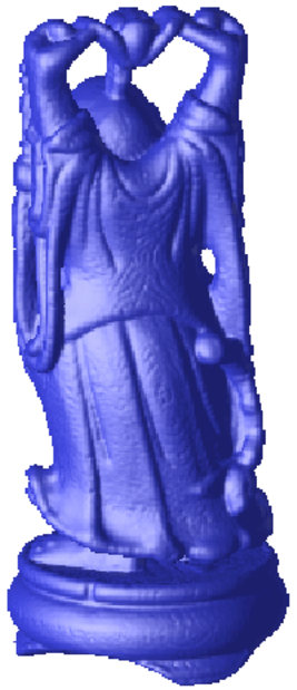
As the last example, we present an application of the distance function in computer visualization. In 20, efficient algorithms are developed to analyze and visualize large sets of unorganized points using the distance function and distance contours. In particular, an appropriate distance contour can be extracted very quickly for the visualization of the data set, which avoids sorting out complicated ordering and connections among all data points. Figure 6.5 shows the visualization of a Buddha statue using a distance contour on a $156\times 371\times 156$ grid from points obtained by a laser scanner. The data set has 543,652 points and is obtained from The Stanford 3D Scanning Repository. The whole process takes a few seconds due to the fast computation of the distance function.

Figure 2.1.

The fast sweeping algorithm in one dimension.

Figure 2.1(a)

the computed distance function after the first left to right Gauss-Seidel sweeping

Figure 2.1(b)

the computed distance function after the second right to left Gauss-Seidel sweeping

Figure 2.2.

The fast sweeping algorithm in two dimensions.

Figure 2.2(a)

the fast sweeping algorithm for a single data point

Figure 2.2(b)

the fast sweeping algorithm for a circle

Figure 4.1.

Figure 4.1(a)

order of dependence in the first quadrant

Figure 4.1(b)

quadrant partition for an arbitrary data point

Figure 4.2.

The numerical solution for two data points $\mathbf{x}_{1},\mathbf{x}_{2}$

Figure 4.3.

Figure 4.3(a)

error at the cell boundary and its propagation

Figure 4.3(b)

domain of dependence of a grid point

Figure 5.1.

Division of a characteristic curve for a general Eikonal equation.

Table 6.1.

Table 6.1(a)

initial setup

100	100	100	100	100	100	100
100	0	100	100	100	100	100
100	100	100	100	100	100	100
100	100	100	100	100	100	100
100	100	100	100	100	100	100
100	100	100	100	0	100	100
100	100	100	100	100	100	100

Table 6.1(b)

after 1st sweep

2	1	1.707	2.545	3.442	4.338	5.192
1	0	1	2	3	3.893	4.673
100	1	2	3	3	3.442	4.048
100	100	100	3	2	2.545	3.252
100	100	100	2	1	1.707	2.545
100	100	100	1	0	1	2
100	100	100	100	1	2	3

Table 6.1(c)

after 2nd sweep

1.707	1	1.707	2.545	3.442	4.338	5.192
1	0	1	2	3	3.893	4.673
1.707	1	1.707	2.707	3	3.442	4.048
3	2	2.925	2.545	2	2.545	3.252
4.371	3.442	2.545	1.707	1	1.707	2.545
4	3	2	1	0	1	2
4.707	3.707	2.707	1.707	1	1.707	2.707

Table 6.1(d)

after 3rd sweep

1.707	1	1.707	2.545	3.442	4.338	5.192
1	0	1	2	3	3.893	4.673
1.707	1	1.707	2.545	2.925	3.416	4.037
2.545	2	2.545	2.545	2	2.545	3.252
3.541	2.925	2.545	1.707	1	1.707	2.545
3.924	2.997	2	1	0	1	2
4.514	3.544	2.545	1.707	1	1.707	2.545

Table 6.1(e)

after 4th sweep

1.707	1	1.707	2.545	3.442	4.338	5.192
1	0	1	2	2.997	3.884	4.668
1.707	1	1.707	2.545	2.925	3.416	4.037
2.545	2	2.545	2.545	2	2.545	3.252
3.416	2.925	2.545	1.707	1	1.707	2.545
3.882	2.997	2	1	0	1	2
4.334	3.441	2.545	1.707	1	1.707	2.545

Table 6.1(f)

after 5th sweep

1.707	1	1.707	2.545	3.441	4.334	5.186
1	0	1	2	2.997	3.882	4.662
1.707	1	1.707	2.545	2.925	3.416	4.037
2.545	2	2.545	2.545	2	2.545	3.252
3.416	2.925	2.545	1.707	1	1.707	2.545
3.882	2.997	2	1	0	1	2
4.334	3.441	2.545	1.707	1	1.707	2.545

Table 6.1(g)

exact distance

1.414	1	1.414	2.236	3.162	4.123	5.099
1	0	1	2	3	4	4.472
1.414	1	1.414	2.236	3	3.162	3.606
2.236	2	2.236	2.236	2	2.236	2.828
3.162	3	2.236	1.414	1	1.414	2.236
4	3	2	1	0	1	2
4.123	3.162	2.236	1.414	1	1.414	2.236

Table 6.1(h)

Voronoi diagram

2	2	2	2	2	2	2
2	2	2	2	2	2	1
2	2	2	2	1	1	1
2	2	2	1	1	1	1
2	2	1	1	1	1	1
1	1	1	1	1	1	1
1	1	1	1	1	1	1

Table 6.2.

maximum change in each sweep

$k=$	1	2	3	4	5	6
$\|u^{k}-u^{k-1}\|_{\infty }$	99	98.293	0.83	0.181	0.007	0

Table 6.3.

distance function to a single data point

Table 6.3(a)

two dimensions

$h=$	0.02	0.01	0.005	0.0025
$\|e\|_{\infty }$	0.04981	0.02440	0.01097	0.00672
$\|e\|_{L^{2}}$	0.02885	0.01386	0.00554	0.00307
$\|e\|_{L^{1}}$	0.02864	0.01371	0.00536	0.00283

Table 6.3(b)

three dimensions

$h=$	0.02	0.01	0.005
$\|e\|_{\infty }$	0.06040	0.02909	0.01429
$\|e\|_{L^{2}}$	0.02496	0.01135	0.00359
$\|e\|_{L^{1}}$	0.02461	0.01111	0.00305

Table 6.4.

distance function to a set of 100 random data points

Table 6.4(a)

two dimensions

$h=$	0.02	0.01	0.005	0.0025
$\|e\|_{\infty }$	0.05565	0.02793	0.01400	0.00693
$\|e\|_{L^{2}}$	0.03385	0.01695	0.00793	0.00366
$\|e\|_{L^{1}}$	0.03310	0.01670	0.00777	0.00357

Table 6.4(b)

three dimensions

$h=$	0.02	0.01	0.005
$\|e\|_{\infty }$	0.06819	0.03355	0.01641
$\|e\|_{L^{2}}$	0.03728	0.01618	0.00673
$\|e\|_{L^{1}}$	0.03772	0.01604	0.00653

Table 6.5.

distance function to a continuous set

Table 6.5(a)

two dimensions

$h=$	0.02	0.01	0.005	0.0025
$\|e\|_{\infty }$	0.05565	0.02793	0.01400	0.00693
$\|e\|_{L^{2}}$	0.03385	0.01695	0.00793	0.00366
$\|e\|_{L^{1}}$	0.03310	0.01670	0.00777	0.00357

Table 6.5(b)

three dimensions

$h=$	0.02	0.01	0.005
$\|e\|_{\infty }$	0.02122	0.01304	0.00783
$\|e\|_{L^{2}}$	0.00381	0.00197	0.00100
$\|e\|_{L^{1}}$	0.00307	0.00159	0.00081

Figure 6.1.

Figure 6.1(a)

contour plot in 2D

Figure 6.1(b)

the contour $u^{h}=0.03$ in 3D

Figure 6.2.

Contour plot of the solution; dotted line is where the boundary condition is prescribed.

Figure 6.3.

Figure 6.3(a)

graph of $f(x,y)$

Figure 6.3(b)

contour plot of the solution (solid line) and $f(x,y)$ (dashed line)

Table 6.6.

$h=$	0.02	0.01	0.005	0.0025
# of iterations	8	8	8	8
$\|e\|_{\infty }$	0.02538	0.01280	0.00644	0.00322
$\|e\|_{L^{2}}$	0.00549	0.00274	0.00137	0.00068
$\|e\|_{L^{1}}$	0.00383	0.00194	0.00097	0.00049

Table 6.7.

maximum difference between two consecutive iterations

iteration	1	2	3	4	5	6	7	8
h=1/200	$10^6$	$10^6$	$10^6$	0.33398	0.01158	0.07068	1.0019x$10^{-6}$	1.0597x$10^{-6}$
h=1/300	$10^6$	$10^6$	$10^6$	0.33781	0.01248	0.07368	1.0101x$10^{-6}$	2.5106x$10^{-6}$
h=1/400	$10^6$	$10^6$	$10^6$	0.33982	0.01299	0.07529	8.8493x$10^{-7}$
h=1/500	$10^6$	$10^6$	$10^6$	0.34107	0.01332	0.07630	7.4581x$10^{-7}$

Figure 6.4.

Figure 6.4(a)

reconstruction of the peak function

Figure 6.4(b)

reconstruction of the hat function

Figure 6.5.

Visualization of 3D scanned points using a distance contour.

Figure 6.5(a)

front

Figure 6.5(b)

diagonal

Figure 6.5(c)

back