Wave-Mean-Flow Interactions in Atmospheric Fluid Flows

Geophysical fluid dynamics describes the flow of gases and liquids in the Earth’s atmosphere, oceans, and other large bodies of water such as lakes and rivers. From a mathematical perspective the evolution of the fluid flow can be described by partial differential equations derived from the physical principles of conservation of mass, momentum, and energy, and including terms that represent the effects of the rotation of the Earth and the effects of buoyancy and gravity. Analyses and solutions of these equations contribute to our understanding of the mechanisms that drive weather over the short term and climate over the long term.

Waves occur naturally in geophysical fluid flows, either in the interior of a body of fluid or at the interface between two fluids such as on the surface of the ocean. The primary mechanisms that generate waves in geophysical flows are the Coriolis force that arises from the Earth’s rotation and the buoyancy and gravitational forces. Wave interactions take place over a wide range of temporal and spatial scales and can have profound effects on the general circulation of the fluid flow. Thus, an understanding of wave properties, including their generation, propagation and interaction with the general circulation, is of great importance for accurate weather forecasting and climate modeling. Forecasting depends on frequent observations and measurements of the properties and current state of the atmosphere, analyses of the data obtained, a good understanding of the dynamics of the atmosphere, the development of mathematical models and computational algorithms, powerful computers, careful analysis and interpretation of the output of the models, and presentation of the output in the form of forecasts.

Mathematical analyses of the fluid equations provide insights that inform the development of the models. Waves may be represented in the equations as perturbations to a suitably averaged background fluid flow. This perspective leads to nonlinear perturbation equations for the wave quantities, which can be linearized and solved exactly in certain special configurations, and can be analyzed in more general situations using the methods of perturbation theory, hydrodynamic stability analysis, and asymptotic analysis. In general, the goal is to understand the wave-mean-flow interactions, i.e., the interchange of energy and momentum between the perturbations and the large-scale background mean flow.

This feature article discusses a mechanism by which certain types of waves interact with a background mean flow in a geophysical fluid context: the critical layer interaction. This type of interaction occurs when a wave propagating with a given phase speed reaches a location called a critical line or critical level, where the speed of the background mean flow is equal to the wave phase speed. In the critical layer surrounding this line, the wave transfers momentum and energy to the background fluid flow, a process called wave absorption, and modifies the flow as a result. This can cause reversal of wind direction, changes in the mean vorticity and temperature, wave breaking, and turbulence. Mathematically, the critical layer corresponds to a singularity in the linearized inviscid equations for steady-amplitude waves.

This article is not intended to be a comprehensive review of atmospheric waves and critical layer phenomena. The focus of the discussion shall be on three types of waves that are ubiquitous in the atmosphere, namely internal gravity waves, planetary Rossby waves, and vortex Rossby waves, and their corresponding critical layer theories. In spite of the differences between the physical characteristics of these waves, there are some similarities in the underlying mathematics and in the approaches used for analyses and for obtaining solutions. The article aims to highlight some of these similarities by referring to critical layer studies of the author and other researchers.

Gravity waves exist in geophysical fluid flows as a result of the competing effects of the downward force of gravity and the upward buoyancy force that causes fluid particles to rise. They include surface gravity waves, such as the familiar water waves that form at the interface between a body of water and the air above.

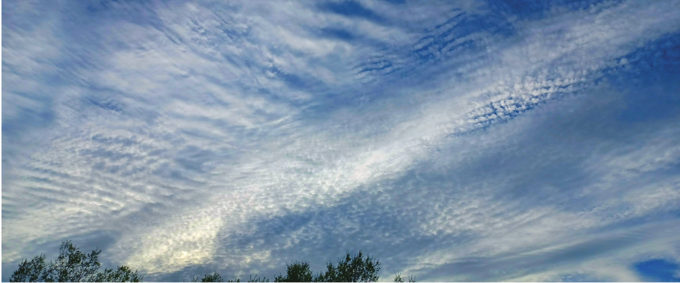
Internal gravity waves occur in the interior of a fluid, e.g., within the atmosphere or within the ocean, and can propagate vertically as well as horizontally. In the atmosphere, the most common examples are orographic waves that are generated by airflow over mountains and other large obstacles and convective waves that form above cloud layers and arise from vertical motion in the lower atmosphere. The spatial scale of these waves is small relative to the planetary scale; their horizontal wavelengths are typically no more than a few hundred kilometers.

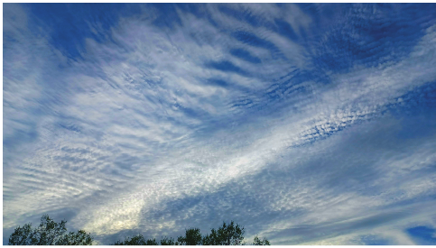
Figure 1 shows an image of gravity waves over stratocumulus cloud layers above the Indian Ocean; they appear as multiple cloud bands corresponding to the troughs and crests of the waves. A similar structure is seen in the clouds in the photograph in Figure 2.

Figure 1.

Gravity wave features over a deck of marine stratocumulus clouds over the Indian Ocean (at about 38.9$^{\circ }$ South, 80.6$^{\circ }$ East): Natural-color image acquired on October 29, 2003, from the Multi-angle Imaging SpectroRadiometer (MISR). From NASA/GSFC/LaRC/JPL, MISR Team. https://earthobservatory.nasa.gov/images/4117/gravity-waves-ripple-over-marine-stratocumulus-clouds

Figure 2.

Gravity wave features in the clouds above Ottawa, Canada, May 13, 2022.

Internal gravity waves have frequent and profound effects on the general circulation of the atmosphere over different time scales and they thus affect both weather and climate. The amplitude of an internal gravity wave tends to increase as the wave propagates upwards. This is because the wave kinetic energy is proportional to the product of the atmospheric density and the square of the amplitude of the fluctuation in the velocity. Conservation of the wave energy in an atmosphere with density decreasing with altitude implies that the wave amplitude increases with altitude. In practice, the rate of increase could be modified by dissipation; this is seen, for example, in the measurements reported by Tsuda Tsu14. The amplitude increase can lead to an instability and possible wave breaking at high altitudes. Moreover, the presence of a critical level acts to filter out the waves, as observed by Whiteway and Duck WD96, and may also lead to breaking. Breaking waves generate the turbulence that is often experienced by air travelers especially when flying over mountain ranges or over convective clouds.

On a longer timescale, internal gravity waves propagating into the stratosphere transfer momentum and energy to the background flow and are known to contribute to the development of the quasi-biennial oscillation (QBO). This is a large-scale oscillation in which the wind direction alternates between eastward and westward phases with a period of 26–30 months. The QBO has profound effects on the stratospheric flow globally, beyond the tropics; it affects the transport and distribution of chemical constituents in the atmosphere and may even affect the strength of hurricanes B$^{+}$01. Given the important role that atmospheric gravity waves are known to play in such weather and climate events, it is important to represent and simulate them accurately in the general circulation models that are used for weather prediction and climate modeling. Historically, this presented a challenge due to their relatively small wavelengths and short time periods. The development of the mathematical theory of gravity waves, including critical layer interactions, has contributed to our understanding of their effects on the general circulation and helped to improve the accuracy of their representation in general circulation models in recent decades FA03.

Rossby waves are oscillations that result from the variation of the rotational or Coriolis force due to the curvature of the Earth. Gravitational and buoyancy effects also play an albeit less significant role in their generation and propagation. These waves play a significant role in weather in the midlatitude regions and are associated with oscillations in the jet stream. Rossby waves are named after the Swedish-born meteorologist Carl-Gustaf Arvid Rossby, who first identified them in 1939 as large-scale wavy patterns in the atmospheric flow and subsequently described their characteristic features. The mathematical theory of Rossby wave critical layers dates back to the 1950s and 60s Lin55. The seminal mathematical studies on the nonlinear inviscid time-dependent problem, presented simultaneously by Stewartson Ste78 and Warn and Warn WW78 in 1978, describe asymptotic solutions that are commonly called the “SWW” solutions. The SWW theory provides insight into the observed formation of the so-called stratospheric “surf-zone,” a large region of planetary wave breaking that extends from northern latitudes towards the tropics MP84.

Rossby waves also exist in the atmosphere on a smaller scale as vortex waves, which take the form of outward-propagating disturbances within cyclonic vortices such as hurricanes Mac68, and result primarily from the force due to the radial gradient of the cyclone vorticity. A hurricane is a cyclone with maximum wind over 32 $\mathrm{ms}^{-1}$ that develops in the atmosphere over the tropical ocean. Typically, a hurricane has a calm area with low atmospheric pressure at its centre. This is called the eye and it is surrounded by a ring of extremely high angular velocity called the primary eyewall. In high-intensity hurricanes, a secondary eyewall sometimes develops as a larger outer ring, increases in intensity and moves inward to replace the primary eyewall. This process repeats as an eyewall replacement cycle. The structure of the vortex at two stages in this process is shown in Figure 3.

Figure 3.

Images captured by the Tropical Rainfall Measuring Mission (TRMM) satellite showing Hurricane Emily as it made landfall in Mexico on July 19 and July 20, 2005. Both images show the rain intensity within the storm. The lowest rain intensities are represented in blue, while the highest intensities are red. https://earthobservatory.nasa.gov/images/15175/hurricane-emily

Vortex Rossby waves interact with the background vortex flow if there is a critical radius where the vortex flow angular velocity is equal to the wave phase speed. The presence of a critical radius affects the structure and intensity of the hurricane and it has been suggested that vortex Rossby waves may contribute to the secondary eyewall development and the eyewall replacement cycle, possibly through a critical radius interaction mechanism MK97.

All these examples underscore the importance of characterizing and understanding atmospheric waves and their behavior at critical layers. This article discusses the critical layer theory for the three types of waves mentioned above. In each case, the discussion is on situations where the wave dynamics is represented in a two-dimensional spatial domain by perturbation equations which are analyzed using asymptotic methods or solved numerically. The focus is on problems involving forced waves, i.e., where an oscillatory boundary condition is applied at one end of the two-dimensional domain and generates a wave with a specified wavelength which propagates into the interior of the region where it encounters a critical layer.

In Section 1 the basic equations of fluid dynamics are presented and perturbation equations are obtained from these. Sections 2–4 give respective overviews of planetary Rossby waves, vortex Rossby waves, and internal gravity waves, and the aspects of their critical layer theories that are similar. Some results of recent numerical studies of the author are presented as illustrations.

1. Geophysical Fluid Flows and Waves

The dynamics of geophysical fluid flows can be described mathematically by equations based on the laws of conservation of mass, momentum, and energy. In a geophysical fluid configuration the flow exists in a three-dimensional domain defined by the spherical Earth, but depending on the spatial scale of the phenomena of interest, we may be able to justify using a two- or three-dimensional representation with Cartesian coordinates as an approximation for spherical geometry.

In terms of Cartesian coordinates $x$, $y$, and $z$, the conservation of mass is written in terms of the fluid density (mass per unit volume) $\rho$, the components $u$, $v$, and $w$ of the fluid velocity in the respective directions, and the time $t$, as the continuity equation

$$\begin{equation} \frac{{ \partial } \rho }{{ \partial t}} + \frac{ \partial }{ \partial x} (\rho u) + \frac{ \partial }{ \partial x} (\rho v) + \frac{ \partial }{ \partial x} (\rho w) = 0. \end{equation}$$

The special case of an incompressible flow, where the rate of change of the density along fluid parcel trajectories is considered to be zero, gives a simplified form of the continuity equation

$$\begin{equation} \frac{\partial u}{\partial x} + \frac{\partial v}{\partial y} + \frac{\partial w}{\partial z} = 0. \end{equation}$$

The conservation of momentum is given by Newton’s Second Law, which says that the rate of change of the fluid momentum (the mass multiplied by the velocity) in some control volume of fluid is balanced by the sum of any applied forces. Considering a fluid parcel of unit volume moving with velocity components $u$, $v$, and $w$, this can be written as

$$\begin{alignat*}{2} \rho \frac{{ D}u}{{ Dt}} & = \rho \left(\frac{{ \partial } u}{{ \partial t}} + { u} \frac{{ \partial } u}{{ \partial x}} + { v} \frac{{ \partial } u}{{ \partial y}} + { w} \frac{{ \partial } u}{{ \partial z}}\right) & & = {-\frac{\partial p}{\partial x}} +F_x \\ \rho \frac{{ D}v}{{ Dt}} & = \rho \left(\frac{{ \partial } v}{{ \partial t}} + { u} \frac{{ \partial } v}{{ \partial x}} + { v} \frac{{ \partial } v}{{ \partial y}} + { w} \frac{{ \partial } v}{{ \partial z}}\right) & & = {- \frac{\partial p}{\partial y}} +F_y \\ \rho \frac{{ D}w}{{ Dt}} & = \rho \left(\frac{{ \partial } w}{{ \partial t}} + { u} \frac{{ \partial } w}{{ \partial x}} + { v} \frac{{ \partial } w}{{ \partial y}} + { w} \frac{{ \partial } w}{{ \partial z}} \right) &= {- \frac{\partial p}{\partial z} +F_z - g \rho }. \end{alignat*}$$

The differential operator $\frac{D}{Dt}$, defined above, gives the rate of change of a fluid property following a fluid parcel moving with velocity $(u,v,w)$; this is known as the Lagrangian derivative.

The terms on the right-hand side are the forces acting on the fluid: $p$ is the pressure (the force per unit area), the spatial derivatives of $p$ are the components of the pressure gradient force, $F_x$, $F_y$, $F_z$ are the components of the Coriolis force and $g$ is the acceleration due to gravity, which gives a gravitational force that acts downward and thus only appears in the vertical momentum equation. Other forces that could be present in a geophysical flow situation have been omitted here, for example the viscous or frictional force and any forces due to electromagnetic effects.

Given the current state of the fluid flow (at $t=0$) in some specified region in space, and some information about the flow at the boundaries, the goal is to solve the equations to find out its state at a later time (for $t > 0$) within that region. This can be written as an initial-boundary-value problem for the system of partial differential equations. To facilitate mathematical analyses, and in particular, to assess the relative magnitude and importance of the various terms, the equations may be considered in nondimensional form.

In a weakly-nonlinear analysis, waves in a fluid are considered as perturbations to a background mean flow with each fluid flow quantity being written as the sum of its mean and a perturbation which is taken to be of small amplitude relative to the mean flow. In a nondimensional framework, we write a quantity $\varphi _{total}$ as

$$\begin{equation} \varphi _{total}(x,y, z,t) = {\bar{\varphi }}+ \varepsilon {\varphi (x,y, z,t)}, {\tag{1}} \end{equation}$$

where ${\bar{\varphi }}$ is a temporal and spatial average of the total quantity, usually the mean in the horizontal west-east ($x$) direction, and $\varepsilon$ is a small nondimensional constant which gives a measure of the magnitude of the perturbation relative to the background flow quantity. This leads to nonlinear equations for the perturbation quantities, which may be linearized as a first approximation. In the linear equations each perturbation quantity $\varphi$ is considered to be an oscillatory and periodic function in one or more spatial directions or in time, and can be represented using Fourier modes, i.e., combinations of sine and cosine functions written in terms of complex exponential functions.

A wave may reach a location in the fluid flow where the background flow speed is equal to the wave phase speed. In an actual three-dimensional flow, this would, in general, be a surface oriented in three-dimensional space. In a two-dimensional representation, it is a critical line. For planetary Rossby waves propagating on a horizontal plane, it is a critical latitude; for vortex Rossby waves traveling radially outward from the center of a vortex, it is a critical radius; and for gravity waves in a vertical plane, it is a critical level.

In the linearized theory for steady-amplitude waves in a flow with no viscosity, the critical line corresponds to a singularity in the ordinary differential equation for the wave amplitude. However, the singular behavior is a mathematical artifact resulting from the omission of the nonlinear terms and viscous terms and the assumption that the wave amplitude is steady. The methods of asymptotic analysis are useful for obtaining an approximate “inner” solution in the critical layer, which is then matched with the solution in the “outer” region away from the singularity. The inner solution is obtained by restoring the viscous terms to the equations in the critical layer, by considering waves with time-dependent amplitude, or by carrying out a weakly-nonlinear analysis in which the previously neglected nonlinear terms are included but they are considered to be “small” relative to the linear terms. In the nonlinear time-dependent formulation, the methods of multiple-scale analysis are used as well; we introduce a suitably scaled “slow” time variable and obtain a slowly varying solution to complete the description of the solution at late time.

The focus of the discussion here will be on weakly-nonlinear time-dependent solutions of the inviscid equations. The development of nonlinear time-dependent critical layer theory for Rossby waves and internal gravity waves has an extensive history developed over the past 60 years. A brief overview of critical layer theory is given here, along with some illustrative numerical simulations for Rossby waves (Sections 2 and 3) and internal gravity waves (Section 4). Each of the problems discussed is based on a two-dimensional simplification of the full three-dimensional system of conservation laws. In each case, the geometry of the problem is defined as either a horizontal or a vertical plane, to give an approximate representation of the direction of propagation of the type of wave studied. Such two-dimensional studies provide us with insights into the dynamics of the respective types of waves in more realistic three-dimensional situations.

2. Planetary Rossby Waves

In this section, the two-dimensional configuration involving Rossby waves in a barotropic shear flow is discussed. A barotropic fluid flow is one in which the density is a function of the pressure only, so that the surfaces of constant density coincide with the surfaces of constant pressure. In situations where the wave propagation is primarily horizontal, a barotropic flow on a two-dimensional horizontal plane may be a reasonable first approximation for the full three-dimensional representation. On the horizontal plane the density is taken to be constant; thus, mass conservation is described by the incompressible form of the continuity equation.

We consider an inviscid barotropic fluid flow on a horizontal plane defined by Cartesian coordinates $x$, in the west-to-east direction, and $y$, in the south-to-north direction, and described by the momentum and mass conservation equations

$$\begin{align} \frac{\partial u}{\partial t} + u \frac{\partial u}{\partial x} + v \frac{\partial u}{\partial y} = - \frac{1}{\rho }\frac{\partial p}{\partial x} +fv,{\tag{2}}\\ \frac{\partial v}{\partial t} + u \frac{\partial v}{\partial x} + v \frac{\partial v}{\partial y} = - \frac{1}{\rho }\frac{\partial p}{\partial y} -fu,{\tag{3}}\\ \frac{\partial u}{\partial x} + \frac{\partial v}{\partial y} = 0. {\tag{4}} \end{align}$$

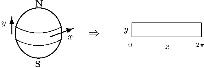
The terms $fv$ and $-fu$ represent the horizontal components of the Coriolis acceleration in the eastward and northward directions respectively, and $f$ is Coriolis parameter, which is defined as $f = 2 \Omega \sin {\theta }$, where $\theta$ is latitude and $\Omega$ is the Earth’s angular velocity. In the $\beta$-plane approximation, the Coriolis parameter is linearized about some reference latitude, say $\theta _0$. The difference in latitude $\theta - \theta _0$ is written in terms of the rectangular coordinate $y$, using the arc length formula, and the Coriolis parameter is approximated by a linear function of $y$. Writing $f \approx f_0 + \beta y$, where $f_0$ is the value of $f$ at $\theta _0$, gives the beta-plane approximation. This approximation is valid for a situation where the latitudinal extent of the domain under consideration is narrow, relative to the scale of the Earth, as shown in Figure 4. Under the beta-plane approximation, a narrow strip like that shown in the diagram, centered at latitude $\theta _0$ is represented by a rectangular domain centered along the line $y=0$ and with periodic boundary conditions in the longitudinal or zonal direction.

Figure 4.

Rectangular configuration for the beta-plane approximation.

The form of the incompressible continuity equation in two variables 4 allows us to define a streamfunction $\Psi (x,y,t)$ by $\frac{\partial \Psi }{\partial y} = -u$, $\frac{\partial \Psi }{\partial x} = v$. This is a function whose level curves in the $xy$-plane define the streamlines, curves which are instantaneously tangent to the velocity vector. The Laplacian of the streamfunction $\nabla ^2 \Psi$ is the vertical component of the vorticity, which measures the extent of local rotation of a fluid parcel at a given location in the flow. Differentiating 2 with respect to $y$ and 3 with respect to $x$ and taking the difference of the resulting equations gives a description of the flow in terms of the streamfunction and vorticity called the barotropic vorticity equation,

$$\begin{equation} \nabla ^2 \Psi _t + \Psi _x \nabla ^2 \Psi _y - \Psi _y \nabla ^2 \Psi _x + \beta \Psi _x =0. {\tag{5}} \end{equation}$$

Here the subscripts $x$, $y$, and $t$ denote differentiation with respect to the respective variables.

The total streamfunction is written in the form suggested by 1. We write

$$\begin{equation*} \Psi (x,y,t) = \bar{\psi }(y) + \varepsilon \psi (x,y,t), \end{equation*}$$

where $\bar{\psi }(y)$ is the basic flow streamfunction, taken as the initial mean in the zonal ($x$) direction, and $\psi (x,y,t)$ is the perturbation streamfunction, and $\varepsilon$ is a “small” parameter that may be considered as $\varepsilon \ll 1$ in an asymptotic analysis. A simple representation of an atmospheric flow is one in which the basic flow has a zonal ($x$) velocity component $\bar{u}(y) = - \bar{\psi }'(y)$ (where the prime denotes the $y$-derivative) and its meridional or latitudinal ($y$) velocity component is zero. This is an example of a shear flow, where the $x$-averaged basic flow speed varies with $y$. This gives a nonlinear equation from which the perturbation quantities can be determined in terms of the specified background flow,

$$\begin{align} \nabla ^{2} \psi _{t} & + \bar{u}(y) \nabla ^{2} \psi _{x} + [\beta - \bar{u}''(y)] \psi _{x} \\ & + \varepsilon (\psi _{x} \nabla ^{2} \psi _{y} - \psi _{y} \nabla ^{2} \psi _{x}) = 0. {\tag{6}} \end{align}$$

If we consider $\varepsilon \ll 1$, we can justify neglecting the nonlinear terms to obtain a linear equation,

$$\begin{equation} \nabla ^{2} \psi _{t} + \bar{u}(y) \nabla ^{2} \psi _{x} + [\beta - \bar{u}''(y)] \psi _{x} = 0. {\tag{7}} \end{equation}$$

Different approaches may be taken to analyze this linear equation, depending on the specification of the background flow and domain and on the information that we wish to obtain about the solutions. In the case where the mean flow speed $\bar{u}$ is constant, equation 7 has constant-amplitude plane wave solutions of the form

$$\begin{equation} \psi (x,y,t) = A e^{i(kx+ly-\omega t)} + \text{c.c.} {\tag{8}} \end{equation}$$

Here $A$ is the complex constant amplitude and “c.c.” denotes the complex conjugate of the function given, so that the wave solution is a real function. The constants $k$ and $l$ are the wavenumbers in the $x$ and $y$ directions, respectively, and define the number of oscillations within an interval of length $2\pi$ and the constant $\omega$ is the wave frequency, which defines the number of oscillations in a time interval of $2 \pi$. This formulation, when substituted into 7 gives the dispersion relation which expresses the frequency as a function of the wavenumbers

$$\begin{equation*} \omega = k \bar{u} - \frac{\beta k}{k^2 + l^2}. \end{equation*}$$

The ratio $c=\omega /k$ is the wave phase speed in the $x$ direction; it gives the speed at which a given phase of the wave, e.g., a crest or trough of the wave, travels in the $x$ direction. Thus, dividing the dispersion relation by $k$ tells us that the phase speed $c$ is always westward (negative) relative to the background flow speed $\bar{u}$. This is a characteristic feature of Rossby waves. Differentiating the dispersion relation partially with respect to $k$ or $l$ gives the $x$ and $y$ components of the group velocity vector

$$\begin{equation*} (c_{gx}, c_{gy}) = \biggl (\frac{\partial \omega }{\partial k}, \frac{\partial \omega }{\partial l}\biggr ), \end{equation*}$$

which defines the direction of propagation of the wave energy. To illustrate the difference between the phase velocity and the group velocity, we may consider a wave packet like that shown in the diagram in Figure 5 propagating in the direction of a horizontal or zonal variable $x$. The $x$-component of the group velocity $c_{gx}$ gives the speed at which the “envelope” of the wave packet, indicated by the dotted curve, travels in the $x$ direction, while $c$ gives the speed of propagation of the crests and troughs of the oscillation. If $c \ne c_{gx}$, as shown in this diagram, then the wave packet is said to be dispersive; this is the case for Rossby waves.

Figure 5.

Propagation of a wave packet profile in a situation where the phase speed $c$ is negative and the $x$-component of the group velocity $c_{gx}$ is positive. The wave packet profile initially takes the form shown in the upper plot, but at later time the wave packet envelope has moved to the right, while the phase has moved to the left.

In the general case with mean flow speed $\bar{u}(y)$, we seek solutions of equation 7 that are periodic and monochromatic in $x$ and $t$ (i.e., with a fixed wavenumber and frequency) and have an amplitude that depends on $y$. This is called the normal mode form, written as

$$\begin{equation} \psi (x,y,t) = \phi (y) e^{ik(x-ct)} + \text{c.c.}, {\tag{9}} \end{equation}$$

where $k$ is the wavenumber, $c$ is the zonal phase speed, $\phi (y)$ is the complex amplitude and as before, “c.c.” denotes the complex conjugate of the function given. The amplitude function $\phi (y)$ satisfies the Rayleigh–Kuo equation,

$$\begin{equation} (\bar{u}(y) - c) [\phi ''(y) - k^2 \phi (y)] + [\beta - \bar{u}''(y)] \phi (y) = 0. {\tag{10}} \end{equation}$$

This is a generalization of the Rayleigh equation, which was first introduced by Lord Rayleigh in the 1880s for the situation with $\beta = 0$.

In the approach of hydrodynamic stability theory, equation 10 is considered in the context of an eigenvalue problem, where $c= c_R + i c_I$ is a complex constant and the solution 9 is thus proportional to $e^{k c_I t}$. The term stability refers to the situation where $c_I \le 0$ and so the amplitude of the perturbation either decays to zero with $t$ or remains constant. We seek to determine the conditions for stability.

The main result obtained from the stability analysis is that if a wave perturbation is unstable, with an amplitude that grows exponentially with $t$, then we must have $\beta - \bar{u}''(y)$ somewhere in the flow. This type of instability is called a barotropic instability. The converse of this result is that if $\beta - \bar{u}''(y)$ is nonzero everywhere in the flow, then the flow is stable to perturbations of the form 9. This is useful information that must be taken into account when we carry out numerical simulations involving barotropic Rossby waves; it is important to ensure that the gradient of the basic flow vorticity $\bar{u}''(y) \ne \beta$ for all $y$ in the domain under consideration in order to avoid barotropic instability. The case with $\beta = 0$ gives Rayleigh’s inflection point theorem which says that the existence of an inflection point in the background flow speed, $\bar{u}''(y)=0$, is a necessary condition for instability.

The Rayleigh–Kuo equation also describes the behavior of forced Rossby waves near a critical line. In the forced wave problem, an oscillatory boundary condition with a specified wave speed $c$ and $x$-wavenumber $k$ is imposed at the one boundary of the spatial domain generating a steady-amplitude travelling wave solution of the form 9. The Rayleigh–Kuo equation describes the variation of the the complex wave amplitude $\phi$ with $y$. The equation has a regular singular point $y=y_c$ where $\bar{u}(y_c) = c$; this corresponds to the critical line. The method of Frobenius is used to obtain a series solution in powers of $(y-y_c)$ and a second solution that includes a logarithmic term of the form $(y-y_c) \log {(y-y_c)}$. For $y < y_c$, the logarithm is defined as

$$\begin{equation*} \log {(y-y_c)} = \log {|y-y_c|} + i \theta , \end{equation*}$$

where the argument $\theta = \pm \pi$. Lin Lin55 showed that the correct branch of the log is given by $\theta =- \mathrm{sgn}(\bar{u}'(y_c))\pi$. This is called a logarithmic phase shift or phase change. Taking this into account in the solutions, we see that there is a discontinuity in the wave amplitude across the critical layer. A wave incident on the critical line from the “north” ($y > y_c$) has its amplitude greatly reduced across the critical layer. The physical interpretation of this is that the wave is absorbed by the background mean flow. In order to represent the wave absorption correctly, however, we need a more realistic model in which the wave amplitude is allowed to vary with $t$ in which case the equation for the wave perturbation is nonsingular.

We consider the forced wave problem in which the solutions of 7 are in the form of waves with time-dependent amplitude

$$\begin{equation} \psi (x,y,t) = \hat{\psi }(y,t) e^{ikx} + \text{c.c.} {\tag{11}} \end{equation}$$

This leads to an initial-boundary-value problem for a partial differential equation involving $t$ and $y$ derivatives of the amplitude function $\hat{\psi }$. Dickinson Dic71 and Warn and Warn WW76 carried out time-dependent analyses using a Laplace transform to find an outer solution, valid for large $t$, and then asymptotic matching to find an inner critical layer solution. They showed that for large $t$ the solution approaches a state with a quasi-steady amplitude with similar features to the steady-amplitude state analyzed earlier by Lin Lin55, namely the same logarithmic phase shift and the corresponding reduction of the wave amplitude across the critical layer. In the inner region, however, the solution grows with time and it becomes apparent that consideration of the neglected nonlinear terms is needed in order to avoid this secular behavior WW76.

Stewartson Ste78 and Warn and Warn WW78 continued the time-dependent investigations by considering the nonlinear equation 6. The nonlinear “SWW” solution, as it is commonly called, behaves like the linear solution at early time in the sense that there is a reduction in the wave amplitude across the critical layer. This reduction is balanced by a transfer of momentum to the mean flow indicating that the wave is indeed absorbed by the mean flow, as the linear solutions suggest. In the nonlinear formulation, the wave absorption results in a wave-induced mean flow acceleration in the vicinity of the critical line. An equation that describes how the mean flow velocity changes in time as a result of the wave interaction is obtained by taking the $x$-average of the $x$-momentum equation 2 over one $x$-wavelength. In 2 $u$ represents the total $x$-component of the velocity, which is equal to the background flow $\bar{u}(y)$ plus the order $\varepsilon$ perturbation, and $v$ represents the $y$-component of the velocity, which is of order $\varepsilon$. Thus, the nonlinear terms involve products of the perturbations which are of order $\varepsilon ^2$. Defining the change in the mean flow velocity as $u_0(y,t)$, we obtain

$$\begin{equation} \frac{\partial u_0}{\partial t} = -\varepsilon ^2 \frac{\partial \overline{u v}}{\partial y}. {\tag{12}} \end{equation}$$

The “over-bar” on the right-hand side denotes the $x$-average taken over one $x$-wavelength and $u$ and $v$ are the $x$- and $y$-components of the wave velocity, $u=-\psi _y$, $v=\psi _x$. The $x$-averaged quantity $\overline{u v}$ is the mean meridional ($y$) momentum flux. In the absence of a critical line, this quantity would be approximately constant, so its $y$ derivative would be small and there would be no significant change in the mean velocity over time. In a configuration with a critical line, there is a large change in the momentum flux in the $y$-direction across the critical layer. As a result the $y$-derivative of the momentum flux on the right-hand side of 12 is large in the vicinity of the critical layer and there is a corresponding change $u_0$ in the the mean flow velocity. There is a corresponding change in the wave energy across the critical layer as energy is transferred from the wave modes to the mean flow.

Over time, additional nonlinear features develop in the critical layer. At late time momentum and energy from the mean flow are transferred to the wave modes as the wave is “reflected” by the mean flow. The timescale on which these nonlinear effects develop depends on the parameter $\varepsilon$ which defines the amplitude of the perturbation relative to the mean flow. Larger amplitude waves evolve into a nonlinear reflecting state sooner. For sufficiently large $\varepsilon$, the system may evolve into a state of over-reflection where the reflection of momentum and energy is greater than the absorption WW78 and then subsequently continue over the long term to alternate between states of net-absorption and over-reflection Bél76 and ultimately to a limiting state of perfect reflection KM85.

Contour plots of the total vorticity, calculated from the asymptotic solutions Ste78WW78 and from numerical solutions Bél76Cam04, show closed contours known as “cat’s eyes” in the critical layer, that eventually overturn and break. Figure 6 shows a contour plot of overturning vorticity contours in a nonlinear Rossby wave critical layer. This result was obtained from a time-dependent numerical solution of 6 in a rectangular domain given by nondimensional variables $0 \le x < 2 \pi$, $-5 \le y \le 5$. A Fourier spectral representation was used in the $x$ direction and a finite difference approximation in the $y$ direction Cam04. In this nondimensional formulation, all the functions and variables in the problem are defined by scaling the dimensional quantities using reference length and timescales that could reasonably describe atmospheric Rossby wave development. The background zonal-mean velocity is chosen as $\bar{u}(y) = \tanh {y}$ and the nondimensional parameter $\beta$ is set to $1$; these choices guarantee that $\beta - \bar{u}''(y) \ne 0$ over the interval of $y$ and prevent the development of a barotropic instability. The waves are forced with a wavenumber of $k=2$ and a phase speed of $c=0$ at the upper boundary of the domain, $y=5$, and propagate towards a critical line located at $y=0$ where $\bar{u} =0=c$. This two-dimensional configuration gives a representation of planetary Rossby waves forced at northern latitudes, propagating horizontally southwards and encountering a critical latitude.

Figure 6.

Wave vorticity $\nabla ^2 \psi (x,y,t)$ in the critical layer at nondimensional time $t=35$ from a numerical solution of equation 6 with nondimensional parameters $\varepsilon = 0.02$, $k=2$.

The change in the mean flow velocity is computed numerically as $u_0(y,t) = \varepsilon \hat{u}(0, y,t)$, where $\hat{u} (\kappa , y,t)$ is the Fourier transform of the $x$-component of the wave velocity, and $\hat{u}(0, y,t)$ is the Fourier component corresponding to the zero wavenumber $\kappa = 0$. Figure 7 shows $u_0(y,t)$ as function of $y$ for fixed $t$. The peak in the magnitude of $u_0$ close to the critical value of $z=0$ is due to the wave-mean-flow interaction which is seen in Figure 6. These results bear a resemblance to the characteristic features of waves that break and result in an acceleration of the background mean flow in the northern stratospheric surf zone MP84.

Figure 7.

Wave-induced mean flow velocity $u_0(y,t)$ as a function of $y$ at nondimensional time $t=35$ from a numerical solution of equation 6 with nondimensional parameters $\varepsilon = 0.02$, $k=2$.

3. Vortex Rossby Waves in a Tropical Cyclone

Vortex Rossby waves also exhibit critical layer interactions which can modify the background flow. Although they differ greatly from planetary Rossby waves with respect to their scale, their structure, and the mechanisms that generate them, there are nevertheless strong qualitative similarities between their critical layer behavior and that of planetary Rossby waves. The development of vortex wave critical layer theory is more recent; in particular, in the past 25 years there have been a number of investigations into the linear initial value problem on a horizontal plane, with constant Coriolis parameter, e.g., BM02MK97. More recently, we NC15aNC15b examined a forced wave problem in a configuration analogous to the SWW problem, where the waves are forced by a oscillatory boundary condition at one end of the domain and propagate towards a critical layer.

In our configuration, we consider a background vortex flow with steady uniform rotation in an annular domain given by $r_1 < r < \infty$, $0 \le \lambda < 2 \pi$. The radius $r_1$ is taken to be the inner eyewall of the vortex. The vortex flow velocity has an azimuthal ($\lambda$) component of $\bar{v}(r)$ and a zero radial ($r$) component, and its angular velocity is $\bar{\Omega }(r)= \bar{v}(r)/r$. This is a simple barotropic approximation for a cyclone like what is shown in Figure 3. A radially symmetric oscillatory boundary condition with a specified frequency $\omega$ and wavenumber $k$ is imposed at $r=r_1$ and generates a wave perturbation of the form

$$\begin{equation} \psi (r, \lambda ,t) = \phi (r) e^{i(k \lambda - \omega t)} + \text{c.c.} \tag{13} \end{equation}$$

The wave propagates radially outwards until it reaches a critical radius, $r=r_c$, where $\bar{\Omega }(r_c) = \omega /k$. We considered a special choice of mean flow angular velocity profile in the form of quadratic function of $r$, which was suggested by BM02. The equations include the “beta-effect,” i.e., the terms involving the parameter $\beta$ which model the effects of the Coriolis force, as well as the nonlinear terms, which are multiplied by the parameter $\varepsilon$. Thus, the problem is governed by two parameters $\beta$ and $\varepsilon$, and the behavior of the solutions depends on their relative magnitude.

The quadratic profile considered for the mean flow angular velocity gives steady-amplitude solutions of the linearized perturbation equation in terms of hypergeometric functions. These solutions show behavior that is similar to that of planetary Rossby waves in the analogous steady-amplitude configuration Lin55: the amplitude of the perturbation is attenuated at the critical radius and there is a logarithmic phase change of $-\pi$. The configuration in which the wave amplitude varies with time $t$ gives linear and nonlinear problems analogous to the planetary Rossby wave critical layer problems studied by Warn and Warn and others Dic71Ste78WW76WW78. Following a similar procedure, using a Laplace transform and asymptotic matching, we are able to obtain linear asymptotic solutions with time-dependent amplitude, valid for large $t$, in the outer region and in the inner region near the critical radius, first for the case with constant Coriolis parameter ($\beta =0$) NC15a. In this case, the linear outer solution approaches a steady state in the limit of infinite time, but the inner solution has secular terms that grow with time. The is an indication that the nonlinear terms and the beta-effect terms need to be considered as well.

A weakly-nonlinear analysis of the nonlinear time-dependent problem, with the beta-effect included, reveals certain aspects of the solutions that bear resemblance to the observed features of the secondary eyewall replacement cycle in tropical cyclones NC15b. In particular, there is an inward displacement of the location of the critical radius with time and additional rings of high wave activity develop corresponding to the critical radii of the components of the solution that arise from the beta-effect.

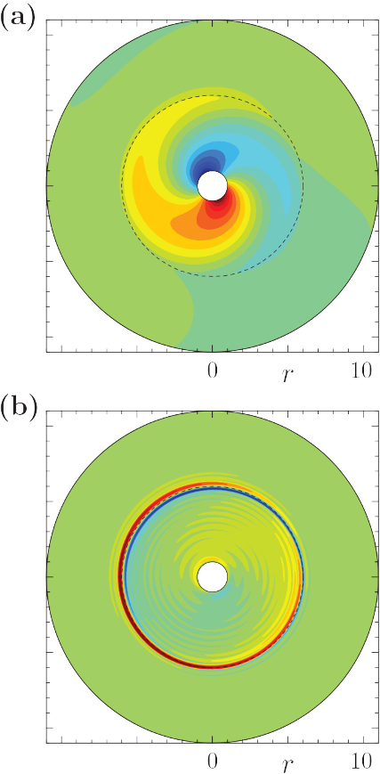
Some numerical solutions for this configuration are shown in Figure 8: the wave streamfunction $\psi (x,z,t)$ in Figure 8(a) and the wave vorticity $\nabla ^2\psi (x,z,t)$ in Figure 8(b). The contour plot of the streamfunction shows that the wave forced at the inner boundary of the annular domain with a wavenumber of $k=1$ propagates radially outwards and its amplitude is reduced at the critical radius, which is indicated by the dashed circle. At this time, a very thin ring of high vorticity has developed in the vicinity of the critical radius resembling a secondary eyewall. This is analogous to the situation of overturning vorticity contours for the related planetary Rossby wave configuration, shown in Figure 6, which was first seen in the SWW asymptotic and numerical solutions Bél76Ste78WW78. In this vortex Rossby waves configuration as well, we found that higher wavenumber components develop with time; however, the low wavenumber components continue to dominate even at late time. This conclusion is consistent with the observations of Hurricane Gloria (1998) which are analyzed and discussed by Shapiro and Montgomery SM93.

Figure 8.

(a) Wave streamfunction and (b) wave vorticity for a wavenumber-$1$ forcing with $\varepsilon = 0.1$ on a $\beta$-plane with $\beta =0.05$. The dashed curve indicates the critical radius for the forced wave. The contour levels are evenly spaced over the interval of values of each function with blue indicating negative values and red indicating positive values.

4. Internal Gravity Wave Packet Generated by an Isolated Mountain

In this section we give an overview of linear and nonlinear critical layer problems for internal gravity waves in a two-dimensional configuration. Internal gravity waves affect the general circulation of the atmosphere through critical level interactions and through wave breaking and saturation. Gravity wave saturation occurs when a wave propagating upwards in the atmosphere reaches a level where its amplitude becomes too large to be sustained and the wave breaks partially to reduce its amplitude and maintain stability. Given the relatively short wavelengths of gravity waves, historically, general circulation models have had difficulty in resolving them adequately and correctly representing the drag force that results from gravity wave critical layer and saturation effects. Consequently, the need to develop and understand the mathematical theory of atmospheric gravity waves has been recognized for many decades.

Gravity wave critical layer theory, in particular, has a rich history that dates back to the 1950s and which developed in parallel to that of planetary Rossby waves. Because they propagate vertically as well as horizontally, the simplest two-dimensional model for gravity waves would be in a vertical plane with one horizontal coordinate tangent to the curved surface of the Earth and one vertical coordinate, normal to the tangent plane.

To a first approximation, the viscous and heat-conduction terms in the momentum and energy conservation equations may be omitted, but just as in the Rossby wave problems, in order to deal with singular solutions and secular terms in the critical layer context, we need to restore these terms to the equations, at least in the inner region, or alternatively consider a time-dependent linear or nonlinear formulation. As in sections 2 and 3, the discussion here will focus on situations with the viscous or heat-conduction terms omitted.

In addition, the Boussinesq approximation is often used to simplify the equations, making them more tractable to mathematical analyses and solutions, while still representing the vertical stratification of the fluid density and temperature. In this approximation, the fluid density is replaced by a background density $\bar{\rho }$ everywhere in the equations, except in the term involving the gravitational force, and the variation of the background density with altitude is considered to be small enough that terms proportional to its vertical derivative are neglected. Under the Boussinesq approximation, there is a linear relationship between the temperature and the density and this allows us to write the energy conservation equation in a simplified form in terms of the density. Moreover, the continuity equation can be written in its simplified incompressible form

$$\begin{equation} \frac{\partial u}{\partial x} + \frac{\partial w}{\partial z} = 0. {\tag{14}} \end{equation}$$

This is analogous to 4, but in terms of one horizontal variable and one vertical variable, rather than two horizontal variables. Again, this two-dimensional continuity equation allows us to define a streamfunction, but in this case it is given by $\frac{\partial \Psi }{\partial z} = -u, \quad \frac{\partial \Psi }{\partial x} = w$.

Differentiating the $x$-momentum equation by $z$ and the $z$-momentum equation by $x$ and taking the difference of the resulting equations gives an equation in streamfunction-vorticity form, which includes the effect of the gravitational force:

$$\begin{equation*} \left( \frac{\partial }{\partial t} + u \frac{\partial }{\partial x} + w \frac{\partial }{\partial z} \right) \nabla ^2 \Psi + \frac{g}{\bar{\rho }} \frac{\partial \rho }{\partial x} = 0. \end{equation*}$$

Here the Laplacian $\nabla ^2\Psi$ is the component of the vorticity in horizontal direction, perpendicular to the vertical plane. The total streamfunction is written in the form 1 as

$$\begin{equation*} \Psi (x,z,t) = \bar{\psi }(z) + \varepsilon \psi (x,z,t), \end{equation*}$$

where $\bar{\psi }(z)$ is the basic flow streamfunction, taken as the initial mean in the horizontal ($x$) direction, and $\psi (x,z,t)$ is the perturbation streamfunction, with $\varepsilon$ again being a small parameter. The basic flow is a shear flow with a horizontal ($x$) velocity component $\bar{u}(z) = - \bar{\psi }'(z)$ (where the prime now denotes the $z$-derivative), and a vertical ($z$) velocity component of zero. This gives a nonlinear equation for the streamfunction and vorticity perturbations and a similar substitution for the total density gives a nonlinear equation for the density perturbation,

$$\begin{align} \nabla ^{2} \psi _{t} + \bar{u}(z) \nabla ^{2} \psi _{x} - \bar{u}''(z) \psi _{x} + g(\bar{\rho })^{-1} \rho _x & \\ + \varepsilon (\psi _{x} \nabla ^{2} \psi _{z} - \psi _{z} \nabla ^{2} \psi _{x}) = 0, &{\tag{15}}\\ \rho _{t} + \bar{u}(z) \rho _{x} + \bar{\rho }'(z)\psi _{x} + \varepsilon (\psi _{x} \rho _{z} - \psi _{z} \rho _{x}) = 0. & {\tag{16}} \end{align}$$

Neglecting the terms involving $\varepsilon$ linearizes equations 15 and 16. We can then combine the linear equations, thus eliminating the terms involving the density perturbation $\rho$ to give a single equation that is second-order in $t$,

$$\begin{align} \left(\frac{\partial }{\partial t} + \bar{u} \frac{\partial }{\partial x}\right)^2 \nabla ^{2} \psi _{x} - \bar{u}''(z) \left(\frac{\partial }{\partial t} + \bar{u} \frac{\partial }{\partial x}\right)\psi _{x} \\ +N^2 \psi _{xx} = 0. {\tag{17}} \end{align}$$

The constant $N$, known as the Brunt–Väisälä frequency or buoyancy frequency, is defined by

$$\begin{equation*} N^2 = - \frac{g}{\bar{\rho }} \frac{d\bar{\rho }}{dz} \end{equation*}$$

and gives a measure of the extent of stratification of the density.

The problems defined by equations 15–17 share some similar features with the corresponding Rossby wave problems described in Section 2. All the approaches for analysis described in Section 2 can be applied here as well. If we consider both the mean flow speed $\bar{u}$ and the Brunt–Väisälä frequency to be constant, then equation 17 has constant-amplitude plane wave solutions of the same form as 8. In this case, we write

$$\begin{equation} \psi (x,z,t) = A e^{i(kx+mz-\omega t)} + \text{c.c.} \tag{18} \end{equation}$$

where the horizontal and vertical wavenumbers are denoted, respectively, by $k$ and $m$. When substituted into 17, this gives the dispersion relation for the wave frequency $\omega$ as a function of the wavenumbers,

$$\begin{equation*} \omega = k \bar{u} \pm \frac{Nk}{(k^2 + m^2)^{1/2}}. \end{equation*}$$

Also, in analogy with the Rossby wave problem, the derivatives of the dispersion relation with respect to $k$ and $m$ give the horizontal and vertical components of the group velocity vector which defines the direction of propagation of the wave energy and the waves are dispersive.

In the general case with mean flow speed $\bar{u}(z)$, we seek steady-amplitude normal mode solutions of equation 17, written as

$$\begin{equation} \psi (x,z,t) = \phi (z) e^{ik(x-ct)} + \text{c.c.}, \tag{19} \end{equation}$$

where $k$ is the wavenumber, $c$ is the zonal phase speed, $\phi (y)$ is the complex amplitude, and as before, “c.c.” denotes the complex conjugate of the function given.

The amplitude function $\phi (z)$ satisfies the Taylor–Goldstein equation,

$$\begin{equation} \phi ''(z) + \left[\frac{N^2}{(\bar{u}(z)-c)^2} - \frac{\bar{u}''(z)}{(\bar{u}-c)} - k^2 \right]\phi =0, {\tag{20}} \end{equation}$$

which is the analog of the Rossby wave Rayleigh–Kuo equation 10 for gravity waves.

As noted in Section 2, the Rayleigh–Kuo theorem gives us a necessary condition for stability of normal mode solutions 9 of 10. The analogous stability theorem for the gravity wave configuration gives a condition in terms of the Richardson number of the background flow. The Richardson number is a function of $z$ which measures the relative effects of the stratification, given by the buoyancy frequency $N$, and the shear, given by the vertical derivative $\bar{u}'(z_c)$ of the mean flow velocity. It is defined as

References

- [Bél76]
- M. Béland, Numerical study of the nonlinear Rossby wave critical level development in a barotropic zonal flow, J. Atmos. Sci. 33 (1976), 2026–2078.
- [B01]
- M. Baldwin et al., The quasi-biennial oscillation, Reviews of Geophysics 39 (2001), 179–229.
- [BB67]
- J. R. Booker and F. P. Bretherton, The critical layer for gravity waves in a shear flow, J. Fluid Mech. 27 (1967), 513–539.
- [BM02]
- G. Brunet and M. T. Montgomery, Vortex Rossby waves on smooth circular vortices, Part I: Theory, Dyn. Atmos. Oceans 35 (2002), 153–177.
- [BS82]
- S. N. Brown and K. Stewartson, On the nonlinear reflection of a gravity wave at a critical level. II, III, J. Fluid Mech. 115 (1982), 217–230, 231–250, DOI 10.1017/S002211208200072X. MR648829Show rawAMSref
\bib{MR0648829}{article}{
author={Brown, S. N.},
author={Stewartson, K.},
title={On the nonlinear reflection of a gravity wave at a critical level. II, III},
journal={J. Fluid Mech.},
volume={115},
date={1982},
pages={217--230, 231--250},
issn={0022-1120},
review={\MR {648829}},
doi={10.1017/S002211208200072X},
label={BS82},
}
Close amsref.✖ - [Cam04]
- L. J. Campbell, Wave-mean-flow interactions in a forced Rossby wave packet critical layer, Stud. Appl. Math. 112 (2004), no. 1, 39–85, DOI 10.1111/j.1467-9590.2004.01587.x. MR2032316Show rawAMSref
\bib{MR2032316}{article}{
label={Cam04},
author={Campbell, L. J.},
title={Wave-mean-flow interactions in a forced Rossby wave packet critical layer},
journal={Stud. Appl. Math.},
volume={112},
date={2004},
number={1},
pages={39--85},
issn={0022-2526},
review={\MR {2032316}},
doi={10.1111/j.1467-9590.2004.01587.x},
Close amsref.✖ - [CM03]
- L. J. Campbell and S. A. Maslowe, Nonlinear critical-layer evolution of a forced gravity wave packet, J. Fluid Mech. 493 (2003), 151–179, DOI 10.1017/S0022112003005718. MR2017947Show rawAMSref
\bib{MR2017947}{article}{
label={CM03},
author={Maslowe, S. A.},
title={Nonlinear critical-layer evolution of a forced gravity wave packet},
volume={493},
date={2003},
pages={151--179},
review={\MR {2017947}},
doi={10.1017/S0022112003005718},
Close amsref.✖ - [CN14]
- L. J. Campbell and L. V. Nikitina, Weakly non-linear analysis of small-amplitude internal gravity waves forced by isolated topography, Geophys. Astrophys. Fluid Dyn. 108 (2014), no. 5, 503–535, DOI 10.1080/03091929.2014.903944. MR3250930Show rawAMSref
\bib{MR3250930}{article}{
label={CN14},
author={Nikitina, L. V.},
title={Weakly non-linear analysis of small-amplitude internal gravity waves forced by isolated topography},
journal={Geophys. Astrophys. Fluid Dyn.},
volume={108},
date={2014},
number={5},
pages={503--535},
issn={0309-1929},
review={\MR {3250930}},
doi={10.1080/03091929.2014.903944},
Close amsref.✖ - [Dic71]
- K. Dickinson, The evolution of the critical layer of a Rossby wave, Geophys. Astrophys. Fluid Dyn. 9 (1971), 185–200.
- [FA03]
- D. C. Fritts and M. J. Alexander, Gravity wave dynamics and effects in the middle atmosphere, Rev. Geophys., 41 (2003), 1–64.
- [KM85]
- P. D. Killworth and M. E. McIntyre, Do Rossby-wave critical layers absorb, reflect, or over-reflect?, J. Fluid Mech. 161 (1985), 449–492, DOI 10.1017/S0022112085003019. MR828155Show rawAMSref
\bib{km}{article}{
label={KM85},
author={Killworth, P. D.},
author={McIntyre, M. E.},
title={Do Rossby-wave critical layers absorb, reflect, or over-reflect?},
volume={161},
date={1985},
pages={449--492},
review={\MR {828155}},
doi={10.1017/S0022112085003019},
Close amsref.✖ - [Lin55]
- C. C. Lin, The theory of hydrodynamic stability, Cambridge, at the University Press, 1955. MR0077331Show rawAMSref
\bib{MR0077331}{book}{
label={Lin55},
author={Lin, C. C.},
title={The theory of hydrodynamic stability},
publisher={Cambridge, at the University Press},
date={1955},
pages={xi+155},
review={\MR {0077331}},
Close amsref.✖ - [Mac68]
- N. J. MacDonald, The evidence for the existence of Rossby-like waves in the hurricane vortex, Tellus XX (1968), 138–150.
- [Mil61]
- J. W. Miles, On the stability of heterogeneous shear flows, J. Fluid Mech. 10 (1961), 496–508, DOI 10.1017/S0022112061000305. MR128232Show rawAMSref
\bib{MR0128232}{article}{
label={Mil61},
author={Miles, J. W.},
title={On the stability of heterogeneous shear flows},
volume={10},
date={1961},
pages={496--508},
review={\MR {128232}},
doi={10.1017/S0022112061000305},
Close amsref.✖ - [MK97]
- M. T. Montgomery and R. J. Kallenbach, A theory of vortex Rossby waves and its application to spiral bands and intensity changes in hurricanes, Q. J. R. Meteorol. Soc. 129 (1997), 3223–3338.
- [MP84]
- M. E. McIntyre and T. N. Palmer, The ‘surf zone’ in the stratosphere, J. Atmos. Terr. Phys. 46 (1984), 825–849.
- [NC15a]
- L. V. Nikitina and L. J. Campbell, Dynamics of vortex Rossby waves in tropical cyclones, Part 1: linear time-dependent evolution on an -plane, Stud. Appl. Math. 135 (2015), no. 4, 377–421, DOI 10.1111/sapm.12094. MR3418903Show rawAMSref
\bib{MR3418903}{article}{
label={NC15a},
title={Dynamics of vortex Rossby waves in tropical cyclones, Part 1: linear time-dependent evolution on an $f$-plane},
volume={135},
date={2015},
number={4},
pages={377--421},
review={\MR {3418903}},
doi={10.1111/sapm.12094},
Close amsref.✖ - [NC15b]
- L. V. Nikitina and L. J. Campbell, Dynamics of vortex Rossby waves in tropical cyclones, Part 2: nonlinear time-dependent asymptotic analysis on a -plane, Stud. Appl. Math. 135 (2015), no. 4, 422–446, DOI 10.1111/sapm.12095. MR3418904Show rawAMSref
\bib{MR3418904}{article}{
label={NC15b},
title={Dynamics of vortex Rossby waves in tropical cyclones, Part 2: nonlinear time-dependent asymptotic analysis on a $\beta $-plane},
pages={422--446},
review={\MR {3418904}},
doi={10.1111/sapm.12095},
Close amsref.✖ - [SM93]
- L. J. Shapiro and M. T. Montgomery, A three-dimensional balance theory for rapidly rotating vortices, J. Atmospheric Sci. 50 (1993), no. 19, 3322–3335, DOI 10.1175/1520-0469(1993)050<3322:ATDBTF>2.0.CO;2. MR1238855Show rawAMSref
\bib{sm}{article}{
label={SM93},
author={Shapiro, L. J.},
author={Montgomery, M. T.},
title={A three-dimensional balance theory for rapidly rotating vortices},
journal={J. Atmospheric Sci.},
volume={50},
date={1993},
number={19},
pages={3322--3335},
issn={0022-4928},
review={\MR {1238855}},
doi={10.1175/1520-0469(1993)050<3322:ATDBTF>2.0.CO;2},
Close amsref.✖ - [SM07]
- D. A. Schecter and M. T. Montgomery, Waves in a cloudy vortex, J. Atmos. Sci. 64 (2007), 314–337.
- [Ste78]
- K. Stewartson, The evolution of the critical layer of a Rossby wave, Geophys. Astrophys. Fluid Dyn. 9 (1978), 185–200.
- [Tsu14]
- T. Tsuda, Characteristics of atmospheric gravity waves observed using the MU (Middle and Upper atmosphere) radar and GPS (Global Positioning System) radio occultation, Proc. Jpn. Acad. Ser. B 90 (2014), 12–27.
- [WD96]
- J. A. Whiteway and T. J. Duck, Evidence for critical level filtering of atmospheric gravity waves, Geophys. Res. Lett. 23 (1996), 145–148.
- [WW76]
- T. Warn and H. Warn, On the development of a Rossby wave critical level, J. Atmos. Sci. 33 (1976), 2021–2024.
- [WW78]
- T. Warn and H. Warn, The evolution of a nonlinear critical level, Stud. Appl. Math. 59 (1978), no. 1, 37–71, DOI 10.1002/sapm197859137. MR0483997Show rawAMSref
\bib{MR0483997}{article}{
label={WW78},
author={Warn, T.},
author={Warn, H.},
title={The evolution of a nonlinear critical level},
volume={59},
date={1978},
pages={37--71},
review={\MR {0483997}},
doi={10.1002/sapm197859137},
Close amsref.✖
Lucy J. Campbell is an associate professor of mathematics at Carleton University in Ottawa. Her email address is campbell@math.carleton.ca.
Article DOI: 10.1090/noti2615
Credits
Figure 1 is courtesy of NASA/GSFC/LaRC/JPL, MISR Team.
Figure 3 was produced by Hal Pierce (SSAI/NASA GSFC).
All other figures and photos are courtesy of the author.