Mixing Surfaces, Algebra, and Geometry

Introduction

This article is a written version of the Maryam Mirzakhani lecture, which the author was honored to give at the Joint Mathematical Meetings in May 2022. Mirzakhani was, of course, the first woman and first Iranian to win the Fields medal.

Figure 1.

The first few surfaces: a sphere, a torus, a double torus, and a triple torus.

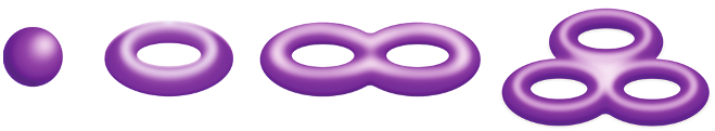
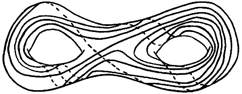
On a basic level, Mirzakhani’s work centers around the geometry of surfaces, as understood through their simple curves. Here, a surface is a 2-dimensional manifold, such as a sphere, a torus, a double torus, etc.; see Figure 1. And a simple curve in a surface is an embedded loop, that is, a path that starts and ends in the same place, never crossing itself. See Figure 2 for an example of a simple curve in the double torus that was drawn by the Fields medalist William Thurston in his research announcement Thu88 (more about his work later).

Starting from this humble-seeming topic, Mirzakhani made surprising and sweeping connections between numerous fields of mathematics, including algebraic geometry, Teichmüller theory, moduli spaces, dynamics, homogeneous spaces, symplectic geometry, and billiards.

Figure 2.

Thurston’s complicated simple curve.

The goal of this article is to explain some recent work on the theory of pseudo-Anosov maps. Informally, a pseudo-Anosov map $f : S \to S$ is a map that mixes the surface $S$ in a complicated way. One way to think about this is that if we start with any simple curve $c$ in $S$, the curves in the sequence $c$, $f(c)$, $f^2(c)$ get more and more complicated, as in Thurston’s picture (for instance, the number of times $f^k(c)$ is forced to pass from the front of the surface to the back will increase exponentially with $k$).

In this article, we will explain three theorems of the author and his collaborators. Along the way, we will connect the theory of pseudo-Anosov maps to number theory, the theory of 3-manifolds, complex analysis, and fluid mixing. Our work is often inspired by and connected to the work of Mirzakhani. Fittingly, we begin by describing a theorem of Mirzakhani that can be viewed as a motivation for the work that follows.

A Motivating Theorem of Mirzakhani

Given a curve on a surface, we can measure its length in a variety of ways. We can endow the surface with a Riemannian metric and compute lengths that way. Or we can fix a projection of the surface to the plane and measure the lengths of the projections (approximately how long is Thurston’s curve in this sense?). Here is a basic question:

Given a particular surface, how many simple curves are there of length at most $L$?

As stated, the answer is easy: infinitely many. Indeed, given a curve with length less than $L$ we can deform it a little bit in order to obtain another curve with length less than $L$ (such a deformation is called a homotopy). A better version of the question is: how many homotopy classes of simple curves are there of length at most $L$?

This question is similar to the classical lattice counting problem: in a ball of radius $L$ in $\mathbb{R}^n$, how many points of the lattice $\mathbb{Z}^n$ are there? In fact, homotopy classes of (simple) closed curves in $T^2$ exactly correspond to (primitive) elements of $\mathbb{Z}^2$. While there is no closed form answer to the lattice question—it depends on the center and the exact value of $L$—we can say the answer is on the order of $L^n$.

If we remove the word “simple,” the answer to the curve question is exponential in $L$ for most surfaces. To see this consider two non-homotopic curves $a$ and $b$ in the double torus with $|a \cap b|$ a single point. We can assume the lengths of $a$ and $b$ are both 1. For every (freely reduced) word of length $L$ in $a$ and $b$ we can construct a (non-simple) curve by following $a$ and $b$ according to the word. The curve will have length at most $L$, hence the exponential growth.

Mirzakhani proved that for simple curves, the answer is strikingly different Mir08. For the statement we denote by $S_g$ the closed surface of genus $g$, so $S_0$ is the sphere $S^2$ and $S_1$ is the torus $T^2$, etc.

Theorem (Mirzakhani).

For $g \geq 2$, the number of simple curves in $S_g$ with length at most $L$ is on the order of $L^{6g-6}$.

Why a polynomial instead of an exponential? Why $6g-6$? A little experimentation will quickly reveal that simple curves are rare: if we choose a random word in $a$ and $b$ as above, we can bet that the resulting curve is not simple. We can try to modify this construction so that only simple curves are produced. That is exactly what Birman and Series did in 1985. In doing so they discovered the lower bound of $L^{6g-6}$ and asked if it was sharp BS85. Mirzakhani’s theorem confirmed this (and much more) using a tour de force of hyperbolic geometry, Teichmüller theory, combinatorics, and dynamics. One upshot of this theorem is that simple curves are special, much in the same way that prime numbers are special.

Taffy Pullers

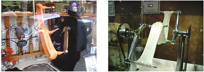
To get into the right frame of mind to study pseudo-Anosov maps, we will begin by investigating a visual (and tasty) way to produce complicated simple curves: taffy pulling. A taffy pulling machine aerates taffy by repeatedly stretching the taffy and folding it. Figure 3 shows two different taffy pulling machines.

Figure 3.

Two taffy pullers.

These pictures, as well as several others in this section, are meant to be viewed as animations. To access the animated versions, visit the following link: https://dmargalit7.math.gatech.edu/mm.shtml.

The taffy puller on the left in Figure 3 has three prongs and the one on the right has four. Which machine is more efficient? How do we even make sense of this question?

We can start to understand the taffy puller on the left by drawing a planar slice of it. If we choose the planar slice to pass perpendicularly through the prongs, we obtain a plane with three dots, one for each prong. We may then draw a simple curve in the plane minus the dots—an imaginary piece of taffy—and trace the evolution of the curve as we run the taffy puller. We want to see how quickly the curve is folding in on itself. If we can quantify that, we will have a sense for how efficient the taffy puller is.

Figure 4.

The effect of the 3-pronged taffy puller on a planar slice of a piece of taffy; in the picture, red dots are prongs and white dots are hinges.

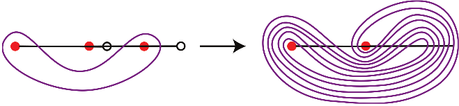
Figure 4 shows what happens to a specific curve under one iteration of the 3-pronged machine (the white dots are hinges, which are not in the plane). To get a handle on the efficiency of this taffy puller we should continue to run the machine and measure the complexity of the resulting curves. The problem, though, is that the pictures are already difficult to draw. It would be hard to draw the curve after two iterations, let alone 10 or 100. What to do?

Thurston’s work on curves gives a solution. One of his many brilliant ideas is to consider the blue object on the top left of Figure 5. This is a graph in the plane with a well-defined tangent line at every point. Thurston calls such a graph a train track.

Figure 5.

Top: deforming a curve towards a train track; bottom: the resulting labeled train track.

What is special about the train track in Figure 5 is that we can take the curve in the figure and push it in a smooth way onto the train track; see the top right of the figure. In other words, we may smoothly deform the curve so that it lies close to the train track and has compatible tangent lines with the train track. We may keep track of the number of “strands” of the curve that pass over each edge (or branch) of the train track. In this way, we obtain a train track with labeled edges, as shown at the bottom of the figure.

We claim that this process loses no information about the curve we started with. Indeed, from the labeled train track, we can recover the curve (up to homotopy) by replacing each branch of the train track with a collection of parallel arcs, the number of arcs being dictated by the label on the branch. The train track then tells us how to glue the arcs together, end to end, to make a curve.

A first observation about labeled train tracks is that most of the labels are redundant. For instance, the 14 must be 14 since this branch is the confluence of branches labeled 10, 2, and 2. This is called the switch condition: at each vertex (or, switch) the sum of the ingoing labels equals the sum of the outgoing labels (the train track is not oriented, and so it is irrelevant which branches we call incoming and outgoing at each switch). The 10 and the 7 are similarly redundant. The end result is that the labels are completely determined by just two: the 5 and the 2.

In this way, labeled train tracks give a succinct way of encoding complicated curves in a surface: for every pair of non-negative integers $x$ and $y$, we obtain a curve based on the blue track; cf. Figure 6. (If $x$ and $y$ are not relatively prime, we obtain a collection of disjoint curves.) In this notation, the curve from the left-hand side of Figure 4 is $(1,0)$. Let us now use this idea to pursue our goal of understanding the image of this curve under iteration of the taffy puller.

Figure 6.

Left: a train track labeled by variables; right: its image under the taffy puller.

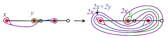
To this end, we take the train track from Figure 5 and we label two of the branches $x$ and $y$ as in the left-hand side of Figure 6. Again, once we label those branches $x$ and $y$, the other branches inherit their own labels. For instance, the branch adjacent to the $x$-branch is labeled $2x$, et cetera.

At this point, the reader should be skeptical: shouldn’t the train track get more and more complicated as we apply the taffy puller? If so, have we really made any progress? Let’s see!

We can apply the taffy puller to the train track from the left-hand side of Figure 6. We obtain the twisted train track shown in the right-hand side of Figure 6, which is indeed much more complicated than the original train track. But then, following Thurston, we observe the following miracle: the twisted train track can be smoothly deformed back onto the original train track. So if we are careful about keeping track of the labels on every branch of the twisted train track, we can re-imagine the twisted train track as the original train track with new labels. The new labels on the $x$- and $y$-branches are $5x+2y$ and $2x+y$. In other words, the taffy puller preserves the blue train track, changing the $x$- and $y$-labels by the matrix

$$\begin{equation*} A = \left( {\begin{array}{cc} 5 & 2 \\2 & 1 \end{array} } \right). \end{equation*}$$

We have converted our topology problem into a linear algebra! We now know that the image of the curve $(1,0)$ under $n$ iterations of the taffy puller is the curve corresponding to the image of $(1,0)$ under $A^n$. For example, the 100th iterate has $xy$-coordinates

$$\begin{equation*} \begin{array}{c} (306455739432329561800579729698332458876\\30954508753693529117371074705767728665, \\1269381235399462048103798648873936844039\\9451028645237163046012909971924256728). \end{array} \end{equation*}$$

By linear algebra we know that the growth rate of these numbers is governed by the eigenvalues of $A$, namely $\lambda = \left(1+\sqrt {2}\right)^2$ and its inverse.⁠¹ Specifically, for large $n$ we have that

¹

The number $1+\sqrt {2}$ is the silver ratio, the growth rate of the Pell sequence: $0, 1, 2, 5, 12, 29, 70, 169, 408, 985, 2378\dots$

✖

$$\begin{equation*} A^{n+1}(v) \sim \lambda \, A^n(v). \end{equation*}$$

For a curve represented by the train track, the magnitude of the corresponding 2D vector is a good measure of the complexity of the curve. Therefore, $\lambda$ is a good measure of the efficiency of the taffy puller. We call this the stretch factor of the taffy puller.

Figure 7.

Left: a curve on a taffy puller; right: the image of the curve and a train track for it.

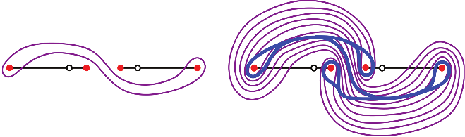
What about the 4-pronged taffy puller? If we play the same game, we can find that the image of the curve on the left-hand side of Figure 7 is the curve on the right-hand side of the figure. We then are led to the train track on the right-hand side of Figure 7. By a similar analysis as in the 3-pronged case, we compute a $3 \times 3$ matrix and find that the stretch factor for the 4-pronged puller is nothing other than $\left(1+\sqrt {2}\right)^2$, the same as for the 3-pronged taffy puller!

This may seem like too much of a coincidence, since these two taffy pullers have little to do with each other, at least on the face of it. So why the same stretch factor? We can give two answers. The first answer is that, in a sense, the two taffy pullers are secretly the same. That is, the pattern of curves we get from the 4-pronged taffy puller is exactly the same as the pattern of curves for the 3-pronged taffy puller, just with an extra red dot thrown in. So in a sense the fourth prong is not actually helping to stretch the taffy(?!).

The second answer is that the number $\left(1+\sqrt {2}\right)^2$ is the smallest possible stretch factor for a taffy puller with three prongs. So this is far from a random number. But why would two different taffy puller designers make taffy pullers with the smallest stretch factor, instead of a larger stretch factor? First, we can always run the taffy puller longer to get larger and larger stretch factors (the stretch factor for the $n$th iterate is $\lambda ^n$). And it stands to reason that when designing a taffy puller the goals are efficiency, simplicity, and elegance. Symmetric/beautiful/efficient patterns tend to give smaller stretch factors. We will return to this idea when we discuss the work of Penner and our work with Farb and Leininger below.

Lest we lose sight of our goal, let us explain what taffy pullers have to do with our main objects of interest, surfaces and homeomorphisms. We may think of an $n$-pronged taffy puller as giving a homeomorphism of a plane with $n$ marked points (equivalently, with $n$ points removed). Through each iteration of the taffy puller we can think of the plane as getting stretched by the motion of the prongs, as though the entire plane was made of a thin layer of taffy; this gives the homeomorphism. So the story developed here is really a story about homeomorphisms of surfaces. We will continue this story in the next section.

If the reader is interested in more about the mathematical history of taffy pullers, we highly recommend the account by Jean-Luc Thiffeault Thi18.

Pseudo-Anosov Maps and the Nielsen–Thurston Classification

In the 1970s, William Thurston proved the following theorem, which gives a classification of surface homeomorphisms into three types Thu88. We will state the theorem first and then explain all of the terms. One thing we will see is that the taffy pullers discussed above can be interpreted as examples of the pseudo-Anosov maps in the theorem. In later sections, we will not often use the precise definition of a pseudo-Anosov map. For a first pass, one should think of a pseudo-Anosov map as one that is similar to a taffy puller in that, asymptotically, it stretches all curves by the stretch factor $\lambda$ as we iterate.

Theorem.

Let $f : S \to S$ be a homeomorphism of a surface. Then $f$ is homotopic to a map $h$ that is either…

1.

periodic: some nonzero power of $h$ is the identity,

2.

reducible: $h$ preserves a nonempty collection of disjoint, essential simple closed curves, or

3.

pseudo-Anosov: $h$ preserves a pair of transverse measured foliations, multiplying the measures by $\lambda$ and $1/\lambda$, respectively.

This is called the Nielsen–Thurston classification because Jakob Nielsen proved many results in this general direction (although pseudo-Anosov maps were not defined prior to Thurston).

We now explain the three types. A periodic homeomorphism should be thought of as a rigid rotation of the surface. The reader might try to imagine some of these, using the pictures of surfaces given above. Different embeddings of a surface in $\mathbb{R}^3$ suggest different periodic maps. (For a challenge: find a period 3 homeomorphism of the double torus $S_2$.)

A reducible homeomorphism is so-called because $h$ restricts to a homeomorphism of the complement of the given collection of curves, and we may think of the resulting map as a simplification (or reduction) of $h$ to a map of simpler surfaces. (Here, a simple curve is essential if it is not homotopic to a point in $S$.)

Before delving into the definition of a pseudo-Anosov map, let us look at an example that you may already be familiar with. Consider the matrix $A = \left( \begin{smallmatrix} 2 & 1 \\ 1 & 1 \end{smallmatrix} \right)$. The matrix $A$ acts on $\mathbb{R}^2$ with two eigenspaces. The eigenvalues of $A$ are $\varphi ^2$ and $1/\varphi ^2$ where $\varphi$ is the golden ratio. Beyond this basic linear algebra, there is an even richer picture to be had: $A$ preserves two foliations of $\mathbb{R}^2$. Each foliation is the collection of lines in $\mathbb{R}^2$ parallel to one eigenspace. We refer to these lines as the leaves of the foliation.

What is more, each of these foliations has a measure, that is, a function that assigns a non-negative real number to each path in $\mathbb{R}^2$ transverse to the given foliation. Specifically, the measure is the total variation of the path in the direction perpendicular to the foliation (so the measure of a path in a leaf of the foliation is zero and the measure of a path perpendicular to the foliation is its Euclidean length). Beyond preserving the two foliations, we can say that $A$ multiplies the measures by $\varphi ^2$ and $1/\varphi ^2$, respectively. So, for instance, if we draw a $1 \times 1$ square with respect to the two foliations for $A$, its image under $A$ will be a rectangle with sides $\varphi ^2$ and $1/\varphi ^2$.

Finally, a pseudo-Anosov homeomorphism of a surface $S$ is a map $f: S \to S$ so that, away from finitely many points of $S$, the action of $f$ looks like (or, is conjugate to) the action on $\mathbb{R}^2$ of a matrix with determinant 1 and two real eigenvalues, such as $A$. As in the Nielsen–Thurston classification there are two measured foliations on $S$ that are preserved by $f$ and whose measures are multiplied by $\lambda$ and $1/\lambda$. The number $\lambda$ is called the stretch factor for $f$.

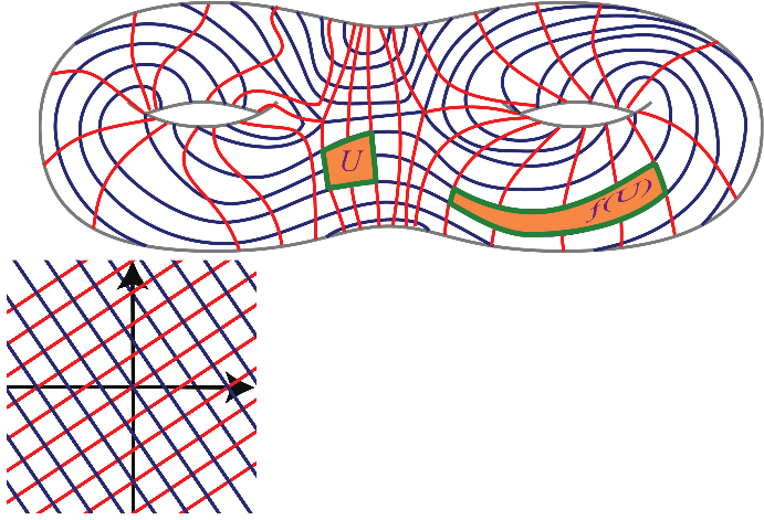
Figure 8 depicts a pair of transverse measured foliations on $S_2$ (to obtain measures, define charts from $S_2$ to $\mathbb{R}^2$ that take the foliations in $S_2$ to foliations of $\mathbb{R}^2$ by lines and pull back natural measures there, as above). We show how a pseudo-Anosov $f$ might distort a square drawn with respect to these foliations.

Figure 8.

Top: a depiction of a pseudo-Anosov map; bottom: two foliations of $\mathbb{R}^2$ preserved by the matrix $A$.

To make a first example of a pseudo-Anosov map on one of the surfaces $S_g$, we observe that the action of $A$ on $\mathbb{R}^2$ descends to a well-defined map $f : T^2 \to T^2$, where the torus $T^2$ is regarded as the quotient $\mathbb{R}^2/\mathbb{Z}^2$. To verify $f$ is well defined, we simply check that for any $(u,v) \in \mathbb{R}^2$ and any $(m,n) \in \mathbb{Z}^2$, we have that $A(u,v)$ and $A(u+m,v+n)$ have the same image in $T^2 = \mathbb{R}^2/\mathbb{Z}^2$ (i.e., the coordinates for $A(u,v)$ and $A(u+m,v+n)$ have the same fractional parts). The map $f$ is locally modeled on $A$: the measured foliations on $\mathbb{R}^2$ descend to measured foliations on $T^2$ and $f$ acts on $T^2$ by preserving the foliations, multiplying the measures by $\lambda = \varphi ^2$ and $1/\lambda = 1/\varphi ^2$.

In the same way that most vectors in $\mathbb{R}^2$ are stretched asymptotically by $\varphi ^2$ by the matrix $A$, curves in $T^2$ have their length stretched asymptotically by $\lambda =\varphi ^2$ as we iterate the pseudo-Anosov map $f$. This is because $f$ is behaving locally like the matrix $A$. This agrees with our observations about taffy pullers, where we saw curves become increasingly more complicated under iteration of the map.

Three Faces

An internet meme (of unclear origin) states:

The Japanese say you have three faces. The first face you show to the world. The second face you show to your close friends and your family. The third face you never show anyone. It is the truest reflection of who you are.⁠²

²

Compare Eli39

✖

We will now discuss three faces of, or ways of thinking about, pseudo-Anosov maps. The three perspectives are increasingly deep and rich, the last being most closely related to the work of Mirzakhani. After discussing the three faces we will aim to understand, from all three perspectives, how we can describe the set of pseudo-Anosov maps with $\log \lambda \leq L$. As we will see, this line of inquiry is analogous to the aforementioned theorem of Mirzakhani, which counts simple curves with length at most $L$.

Face 1: Pseudo-Anosov Maps and the Mapping Class Group

For a surface $S$, the mapping class group $\operatorname {MCG}(S)$ is a quotient of the group of (orientation-preserving) self-homeomorphisms of $S$. Specifically, two homeomorphisms are equivalent if they are homotopic, that is, if one can be deformed to the other in a continuous way. This is a countable group that encodes the symmetries of $S$.

We would be remiss not to mention that the theory of mapping class groups recently celebrated its 100th birthday. The first lecture on the topic was given by Max Dehn in Breslau, Poland, on February 22, 1922.

Today, mapping class groups are connected to many areas of mathematics and science, from physics to dynamics to algebraic geometry to number theory. Here are three of the ways that mapping class groups arise in mathematics (see FM12 for details):

•

The Dehn–Nielsen–Baer theorem says that every automorphism of the fundamental group $\pi _1(S)$ is induced by an element of $\operatorname {MCG}(S_g)$.

•

The Earle–Eells theorem implies that $S_g$-bundles over a space $B$ correspond bijectively to homomorphisms $\pi _1(B) \to \operatorname {MCG}(S_g)$.

•

By the work of Fricke, $\operatorname {MCG}(S_g)$ is the (orbifold) fundamental group of the moduli space of algebraic curves of genus $g$.

The Nielsen–Thurston classification can be regarded as a trichotomy for the mapping class group: a mapping class is considered to be pseudo-Anosov if it has a pseudo-Anosov representative. So this is the first face of a pseudo-Anosov homeomorphism: as an element of $\operatorname {MCG}(S)$.

As we will see, the pseudo-Anosov property of a mapping class has profound implications for the corresponding automorphisms of $\pi _1(S)$, surface bundles, and loops in moduli space.

Face 2: Pseudo-Anosov Maps and 3-Manifolds

The second face of a pseudo-Anosov map—as a mapping torus—is richer than the first. The story begins with the following quote from Thurston Thu01:

It seemed pretty obvious that a 3-manifold that fibers over the circle couldn’t possibly have a hyperbolic structure. I kept trying to think of proofs of that. I kept proving it but then when I went to explain it to somebody the proof had a fallacy…

Let us explain the two technical terms in this quote, “fibers over the circle” and “hyperbolic.” We begin with the former. Given any homeomorphism $f : S \to S$, we may construct a 3-dimensional manifold, called the mapping torus $M_f$, by taking the product $S \times [0,1]$ and gluing the two ends by $f$. More precisely:

$$\begin{equation*} M_f = \left( S \times [0,1] \right) / \sim \end{equation*}$$

where $(x,0) \sim (f(x),1)$ for all $x \in S$. In Thurston’s quote, a 3-manifold that fibers over the circle is nothing other than such a mapping torus.

Next, a manifold is hyperbolic if it admits a Riemannian metric of constant curvature $-1$ (equivalently, if it is a quotient of hyperbolic space). Thurston’s quote, which is from 2001, describes his thinking in the 1970s, when he and others were wondering which 3-manifolds were hyperbolic.

Why would Thurston think that mapping tori could not be hyperbolic? It helps to draw a picture of $M_f$, as in Figure 9. Our illustration of $M_f$ looks at first glance like a direct product $S \times S^1$. And indeed if $f$ is the identity this is the case. When $f$ is not the identity, $M_f$ is a twisted product. To understand this twistedness, we must look inside $M_f$.

Consider the curve $c$ in $S$ shown in the figure. As we push $c$ around the circle direction, it traces out a tube. If $f(c)$ is different from $c$ then the tube does not close up after traveling around the circle direction once and we can keep extending the tube.

Figure 9.

A mapping torus $M_f$ along with a curve $c$, its image $f(c)$, and the tube connecting the two.

On the other hand, if $f$ does preserve a simple closed curve $c$ in $S$, then the tube created by pushing $c$ in the circle direction closes up to give a torus in $M_f$. Similarly, if some nonzero power of $f$ preserves $c$ (even up to homotopy), then we again obtain an (immersed) torus, except now the torus wraps around the circle direction more than once.

Let us circle back to the question of hyperbolicity. It is a fact that a hyperbolic manifold cannot contain an (essential) torus, since a torus is inherently a Euclidean object (the real reason is that the torus would give rise to a $\mathbb{Z}^2$ in $\operatorname {Isom}\mathbb{H}^3$, which does not exist). So by the previous paragraph, if we want $M_f$ to be hyperbolic then no power of $f$ can preserve (the homotopy class of) any simple curve. It might be hard to believe that such an $f$ exists.

But we know better. As with our taffy puller examples, pseudo-Anosov maps have the desired property: no power fixes any simple curve. So at least those $M_f$ have a chance of being hyperbolic. Thurston showed that indeed all of these mapping tori are hyperbolic, that is, $M_f$ is hyperbolic if and only if $f$ is (homotopic to) a pseudo-Anosov map (his argument is fleshed out by Otal Ota96). And so we have the second face of a pseudo-Anosov map, as a hyperbolic mapping torus.

Face 3: Pseudo-Anosov Maps and Moduli Space

The third face of a pseudo-Anosov map is the most challenging (and also the most rewarding): we will see that pseudo-Anosov maps can be regarded as loops in the moduli space $\mathcal{M}(S)$ of complex structures on $S$. Before we get to that, let us first aim to understand what this moduli space is.

A complex structure on $S$ is a way of identifying $S$ with the complex plane $\mathbb{C}$, at least locally. More specifically, we cover $S$ with open sets $U_\alpha$ and choose for each $\alpha$ an embedding $\phi _\alpha : U_\alpha \to \mathbb{C}$ called a chart. The catch is that on the open set $U_\alpha \cap U_\beta$ there are two different charts, $\phi _\alpha$ and $\phi _\beta$, and we insist that the change of coordinates $\phi _\alpha ^{-1} \circ \phi _\beta$ is a biholomorphic map. This definition is analogous to that of a smooth structure. The last condition ensures that the different charts are consistent with one another.

How do we even make a single complex structure on $S$? When $S$ is the torus $T^2$ every complex structure on $S$ is given by a parallelogram $P$ in the complex plane with unit area. We obtain the torus topologically by identifying opposite sides of $P$. The interior of $P$ is then an open set in $T^2 = P/{\sim }$ that is already identified with a subset of $\mathbb{C}$ (the chart is the inclusion map). It is a good exercise to find the other open sets and charts needed to give $T^2$ a complex structure. But since the interior of $P$ is “most” of $T^2$, it should be believable that $P$ gives rise to a (unique) complex structure on $T^2$.

Two complex structures on a surface $S$ are considered to be the same if there is a biholomorphic map from one to the other. For example if we rotate a parallelogram $P$ to obtain a parallelogram $P'$, then $P$ and $P'$ give equivalent complex structures on $T^2$. On the other hand, the complex structure on $T^2$ coming from a square is not equivalent to the one coming from a (non-square) rectangle. Intuitively, this is because holomorphic maps preserve angles, but a map from a square to a rectangle must distort angles.

How do we move around in the moduli space $\mathcal{M}(S)$? Again, let us start with the case $S=T^2$ and in particular at the point in $\mathcal{M}(T^2)$ corresponding to a square. If we deform the square through a continuous family of parallelograms, that gives a continuous deformation of the complex structure on $T^2$, and hence a path in $\mathcal{M}(T^2)$.

We now describe two explicit paths in $\mathcal{M}(T^2)$. For $\tau \in [1,\infty )$ let $P_\tau$ be the unit-area parallelogram with vertices 0, $1/\tau$, $\tau i$, and $1/\tau + \tau i$. When $\tau =1$, the parallelogram $P_\tau$ is a square and otherwise it is a rectangle that gets skinnier as $\tau \to \infty$. Similarly, for $\tau \in [0,\infty )$ let $Q_\tau$ be the unit-area parallelogram with vertices 0, 1, $i+\tau$ and $i + \tau +1$ in $\mathbb{C}$. The parallelogram $Q_\tau$ shears as $\tau$ increases. In both cases, the continuously changing shapes of the parallelograms give continuously changing complex structures on $T^2$, and hence a path in $\mathcal{M}(T^2)$.

Figure 10.

The moduli space of the torus.

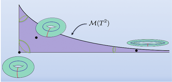
We usually draw $\mathcal{M}(T^2)$ so that it looks like a long and pointy pillowcase, as in Figure 10. It turns out this space is homeomorphic to $\mathbb{R}^2$. (Can you see from the above discussion why it should be 2-dimensional?). There are two special points, corresponding to the complex structures on $T^2$ coming from a square (bottom left of the figure) and a regular hexagon with sides identified (top left of the figure); these are the only two tori with extra symmetry, besides the translational symmetry along the $S^1$ factors (all parallelograms have reflections, but these are not allowed in the complex setting).

The complex structures corresponding to skinny parallelograms are off to the right in the picture; this is the cusp of moduli space, or the part at infinity. The path $P_\tau$ travels off into this region. This region is also called the thin part of moduli space; not because moduli space is thin there (which is also true) but because the tori there are thin.

Figure 11.

The loop $Q_\tau$ in the moduli space of the torus.

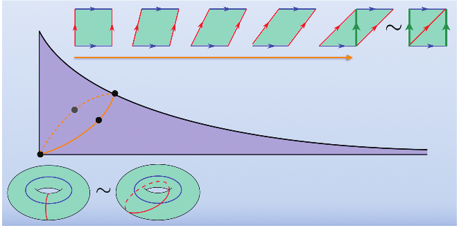
What about $Q_\tau$? Far from traveling into the cusp of moduli space, we claim that $Q_\tau$ is a closed loop. Indeed, we will show that $Q_0$, the square torus, is the same point as $Q_1$, the torus corresponding to a parallelogram with acute angle $\pi /4$. In other words, there is a biholomorphic (or, angle preserving) map from $Q_0$ to $Q_1$. Indeed, if we divide the $Q_1$ parallelogram into two triangles with a vertical line, then we can reassemble those two triangles (respecting identifications) and obtain the square corresponding to $Q_0$. See Figure 11 for an illustration of $Q_\tau$.

Now that we have in hand an example of a loop in moduli space, we can return to our stated goal of relating loops in moduli space to pseudo-Anosov maps. Let us look again at $Q_0$ and $Q_1$. Suppose we decorate the square $Q_0$ by labeling its pairs of opposing sides by $a$ and $b$. As we vary $\tau$ we can take the decorations with us. When we get to $Q_1$, we indeed have a torus that is biholomorphic to the square torus, but the decoration is different: $a$ and $b$ are now at an angle of $\pi /4$. More to the point, $Q_0$ and $Q_1$ differ by a homeomorphism of $T^2$ that fixes $a$ and sends $b$ to the diagonal (this is like a shear in linear algebra).

The previous paragraph gives a correspondence between loops in $\mathcal{M}(T^2)$ and elements of $\operatorname {MCG}(T^2)$. So what does this have to do with pseudo-Anosov maps? It turns out that, for general $S$, pseudo-Anosov maps are exactly the ones that correspond to essential loops in $\mathcal{M}(S)$. There is a natural metric on $\mathcal{M}(S)$, called the Teichmüller metric, which measures the distortion required to get from one complex structure to another, and the loops corresponding to pseudo-Anosov maps are exactly the ones with geodesic representatives in this metric. The length of the loop is $\log \lambda$, where $\lambda$ is the stretch factor.

Small Stretch Factors

We gain insight into a geometric space by understanding the set of lengths of loops, the so-called length spectrum. And one way to probe the length spectrum is to list the smallest elements. Mirzakhani’s theorem above gives a count of the number of short curves on a surface. Since short loops in moduli space correspond to pseudo-Anosov maps with small stretch factor $\lambda$, we would like a similar count of the pseudo-Anosov maps with small stretch factor.

It is a fact that for every surface there is a smallest stretch factor among all pseudo-Anosov maps. Even more, the set of stretch factors has no accumulation points in $\mathbb{R}$, and so it makes sense to talk about the smallest $27$ stretch factors (for example).

So what is this smallest stretch factor? For the torus it is $\varphi ^2 \approx 2.168$, the stretch factor seen above (exercise!). For $S_2$, Cho and Ham proved that the smallest stretch factor is the largest root of the polynomial $x^4-x^3-x^2-x+1$, or about 1.722. See a pattern? Actually, nobody knows the pattern. The smallest stretch factor for $\operatorname {MCG}(S_g)$ is still a mystery for all $g \geq 3$.

While we do not know in general which pseudo-Anosov maps have the smallest stretch factor for each surface we still can, surprisingly, give qualitative descriptions of what they look like.

Penner proved Pen91 there are numbers $c$ and $C$ so that the log of the smallest stretch factor $\lambda _g$ on $S_g$ lies between $c/g$ and $C/g$. We write this as

$$\begin{equation*} \log \lambda _g \approx \frac{1}{g}. \end{equation*}$$

So as the genus increases, the size of the smallest stretch factor gets smaller and smaller, indeed, closer and closer to 1.

Figure 12.

The Penner construction of pseudo-Anosov maps with small stretch factor.

The upper bound $C/g$ is obtained by giving an explicit example $f_g$ of a pseudo-Anosov map on $S_g$ with stretch factor less than $C/g$. Here is (very roughly) how Penner constructs $f_g$. First, he chooses a pseudo-Anosov map $f_2$ on the surface of genus 2 with one boundary component. Since the latter surface lies inside $S_g$ for all $g \geq 3$ we may consider $f_2$ as an element of $\operatorname {MCG}(S_g)$ for all $g \geq 3$. Let $r_g$ be a rotation of $S_g$ by one “click” (a rotation by $2\pi /g$) as in Figure 12. Then $f_g$ is given by the composition

$$\begin{equation*} f_g = r_g \circ f_2. \end{equation*}$$

The map $f_2$ has some stretch factor $\lambda$, and the map $r_g$ does no stretching. So the net effect is that the stretching done by $f_2$ gets dampened out by the rotation, and the amount of dampening increases with $g$, which is the period of $r_g$. Penner shows that if $f_2$ and $r_g$ are chosen very carefully, then the stretch factor of $f_g$ is approximately $\lambda /g$, as desired.

Because of Penner’s theorem, we have the following notion of smallness for a stretch factor. We fix a number $L$ and say that a stretch factor $\lambda$ for a pseudo-Anosov $f : S_g \to S_g$ is small if

$$\begin{equation*} \log \lambda \leq L/g. \end{equation*}$$

By Penner’s theorem, there are small stretch factors for every $g$ as long as $L$ is greater than or equal to the constant $C$ in his theorem.

In the remainder of this article we focus on the question:

What do the small-stretch pseudo-Anosov maps look like, and where do we find them?

We approach this question from the three perspectives on, or three faces of, pseudo-Anosov maps given above.

Connections to Number Theory: Lehmer’s and Fried’s Problems

Fried proved that the stretch factor $\lambda$ for a pseudo-Anosov map is always a bi-Perron unit: it is the root of a monic, integer polynomial, and each algebraic conjugate of $\lambda$ is either equal to $1/\lambda$ or has modulus in $(1/\lambda ,\lambda )$. Fried then posed the following problem: show that every bi-Perron unit is the stretch factor of a pseudo-Anosov map Fri85. It would be remarkable if there was such a strong connection between this number theoretic property of real numbers and the topological property of being a stretch factor.

As of this writing, Fried’s problem is wide open, and there is no convincing evidence either way (Fried considered other basic number theoretic properties, and could not find any more restrictions). The problem is hard because there is no straightforward bridge between the number theory and the topology and no conspicuous place to look for counterexamples.

As for the problem of understanding the smallest stretch factors, there is a famous analogue in number theory. The Mahler measure of a polynomial is the product of the absolute values of the roots that lie outside the unit circle. Lehmer’s problem (or conjecture) is to show that the set of Mahler measures of monic, integer polynomials is bounded away from 1 and further that the minimal such Mahler measure is attained by Lehmer’s polynomial

$$\begin{equation*} x^{10}+x^9-x^7-x^6-x^5-x^4-x^3+x+1. \end{equation*}$$

The Mahler measure of Lehmer’s polynomial is $\mu \approx 1.17628$. Lehmer’s problem has been open since his 1933 paper.

Lehmer’s polynomial appears elsewhere, for instance in Reidemeister’s 1927 manuscript Rei27 as the Alexander polynomial of the $(-2,3,7)$-pretzel knot. For a variety of other connections between Lehmer’s problem and topology, see the papers by Silver–Williams SW07 and by Leininger Lei04.

Face 1: Small Stretch Factors and the Mapping Class Group

By work of Dehn and Lickorish, each $\operatorname {MCG}(S_g)$ is normally generated by a single element FM12, Theorem 4.1. This means for each $g$ there is a single element $f \in \operatorname {MCG}(S_g)$ so that each element of $\operatorname {MCG}(S_g)$ is a product of conjugates of $f$. The specific element given by Lickorish is known as a Dehn twist.

As in linear algebra, we think of conjugate group elements as acting in the same way, just under different sets of coordinates. So we can think of this theorem as saying that there is one type of “move” that allows us to obtain all symmetries of a surface. This is a familiar notion. For instance the fact that the symmetric group $\Sigma _n$ is generated by transpositions and the fact that the special linear group $\mathrm{SL}_n(\mathbb{Z})$ is generated by primitive elementary matrices (elementary matrices with a 1 off the diagonal) are instances of this. Since transpositions are all conjugate in $\Sigma _n$ and primitive elementary matrices are all conjugate in $\mathrm{SL}_n(\mathbb{Z})$, both facts imply that $\Sigma _n$ and $\mathrm{SL}_n(\mathbb{Z})$ are normally generated by a single group element.

Transpositions and elementary matrices are very simple elements: transpositions fix $n-2$ elements of $\{1,\dots ,n\}$, and elementary matrices fix a codimension 1 subspace of $\mathbb{R}^n$. Similarly, a Dehn twist in $S_g$ is the identity outside of an annulus in $S_g$ (the smallest essential subsurface). While it is perhaps not surprising that such simple elements are normal generators, the following question of D. D. Long is more intriguing:

Does $\operatorname {MCG}(S_g)$ have a normal generator that is pseudo-Anosov?

Long answered in the affirmative for $g=1$, but his question was open since 1986 for $g \geq 2$. To get a sense for why this is difficult, try to determine if $B = \left( \begin{smallmatrix} 25 & -29 \\ 19 & -22 \end{smallmatrix} \right)$ is a normal generator for $\mathrm{SL}_2(\mathbb{Z})$. To put it another way, it is natural that the usual row operations (or elementary matrices) suffice to reduce matrices, but much less natural to understand if the complicated “row operations” given by $B$ suffice.

With Lanier, we answered Long’s question in the affirmative LM22. In fact we showed that there are many pseudo-Anosov normal generators.

Theorem (Lanier–Margalit).

If a pseudo-Anosov element of $\operatorname {MCG}(S_g)$ has stretch factor less than $\sqrt {2}$, then it is a normal generator.

Our work builds on previous joint work with Farb and Leininger FLM08. One restatement of the theorem is that if a pseudo-Anosov map has small stretch factor, then it lies outside every proper, normal subgroup of $\operatorname {MCG}(S_g)$ (a normal subgroup contains the normal closures of each of its elements).

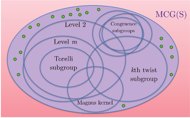
The mapping class group is rich with interesting normal subgroups, some of which are named in Figure 13. The small stretch pseudo-Anosov maps lie outside all of them, as caricaturized in the figure.

Figure 13.

A cartoon of the mapping class group, with the small-stretch pseudo-Anosov maps shown as green dots.

This gives a first answer to our motivating problem of understanding the nature of small-stretch pseudo-Anosov maps. This answer even applies to the set of pseudo-Anosov maps with $\log \lambda \leq L$. For the second and third faces we use the stronger assumption $\log \lambda \leq L/g$.

Face 2: Small Stretch Factors and 3-Manifolds

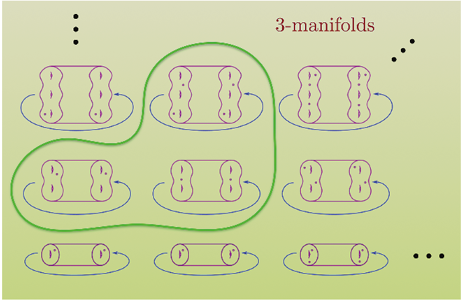
We now turn our attention to the 3-manifold perspective. The starting point is the following fact: there are examples of mapping classes $f \in \operatorname {MCG}(S_2)$ and $h \in \operatorname {MCG}(S_3)$ so that the mapping tori $M_f$ and $M_h$ are homeomorphic. Said another way, there is a single 3-manifold that can be realized as a mapping torus in two very different ways.

While this may seem counterintuitive at first, we can gain insight by subtracting two dimensions. To any element $\sigma$ of the symmetric group $\Sigma _n$ we may make a mapping torus: we multiply the discrete set $\{1,\dots ,n\}$ by the interval $[0,1]$, which gives a disjoint union of $n$ intervals, and then we glue the ends together according to $\sigma$. The end result is a disjoint union of circles, the number of circles being the number of cycles in the cycle decomposition for $\sigma$. From this, we see that we may write the circle as a mapping torus for elements of different permutation groups. The phenomenon in the previous paragraph is simply a higher dimensional analogue.

As in the symmetric group case, we can often realize a single 3-manifold as a mapping torus in infinitely many ways, with underlying surfaces of infinitely many different genera. As mentioned, a deep theorem of Thurston says that a mapping torus is hyperbolic if and only if the gluing map is pseudo-Anosov. Thus, if one of the gluing maps for a mapping torus is pseudo-Anosov, all of them are. In this way, we obtain infinitely many pseudo-Anosov maps, on surfaces of different genera, from a single pseudo-Anosov map.

Even better, McMullen McM00 showed how to use work of Fried to obtain Penner’s asymptotics this way. That is, from a single hyperbolic mapping torus, one can find a sequence of pseudo-Anosov maps $f_i \in \operatorname {MCG}(S_{g_i})$ (as in the previous paragraph) with the $g_i$ tending to infinity, and the logs of the stretch factors of the $f_i$ bounded above by $C/g_i$.

From this starting point, Farb, Leininger, and the author set out to study the set of small-stretch pseudo-Anosov maps from the 3-manifold perspective. Here, we consider the set of pseudo-Anosov maps on all $S_g$ with $\log \lambda$ bounded above by $L/g$ for some fixed $L$. We denote this set by $\Psi _L$.

Our first hope was the set of mapping tori

$$\begin{equation*} \Omega _L = \{ M_f : f \in \Psi _L \} \end{equation*}$$

was finite. This would be a sort of converse to McMullen’s construction: not only does a single mapping torus give Penner’s asymptotics, but all sequences of mapping classes realizing Penner’s asymptotics in turn give a single, or at least finitely many, mapping tori.

Unfortunately, this is not true, and there is an immediate obstruction. When we make a mapping torus from a pseudo-Anosov map $f$, the foliations on the surface give rise to 2-dimensional foliations of $M_f$. The infinitely many pseudo-Anosov maps giving $M_f$ all give the same foliations of $M_f$. The degrees of the singularities for the foliations for $f$ are the same as the degrees of the singularities in $M_f$. But Penner’s examples of small-stretch pseudo-Anosov maps have more and more singularities as $g$ increases (there are singularities at the two fixed points of the rotation $r_g$ in Figure 12, each with degree $g$).

Figure 14.

A cartoon of the infinite world of mapping tori, with the small-stretch pseudo-Anosov maps occurring in the finite set encircled by the green loop.

With Farb and Leininger we proved that this is the only thing that goes wrong with our initial hope FLM11. More precisely, let $\Psi _f^\circ$ be the set of pseudo-Anosov maps of punctured surfaces obtained by deleting the singularities of elements of $\Psi _f$.

Theorem (Farb–Leininger–Margalit).

The set of (non-compact) 3-manifolds

$$\begin{equation*} \Omega _L^\circ = \{ M_f : f \in \Psi _L^\circ \} \end{equation*}$$

is finite.

In other words, up to adding and deleting finitely many singular points, the set of small-stretch pseudo-Anosov maps all come from a finite set of 3-manifolds. Figure 14 gives a caricature.

It is an open problem to determine the cardinality of $\Omega _L^\circ$. Is it ever 1?

The Symmetry Conjecture

With Farb and Leininger we formulated a conjecture that suggests a different way to describe the pseudo-Anosov maps with small stretch factor. In the statement, a partial pseudo-Anosov map $f : S_g \to S_g$ is a map supported on a subsurface $R$ and so that the restriction $f|R$ is pseudo-Anosov (such as $f_2$ above).

Conjecture (Farb–Leininger–Margalit).

There is a function $\xi = \xi (L)$, independent of $g$, with the following property. If $f : S_g \to S_g$ lies in $\Psi _L$, then $f$ is the composition $\rho \circ h$ where $\rho \in \operatorname {MCG}(S_g)$ is periodic and $h \in \operatorname {MCG}(S_g)$ is a partial pseudo-Anosov element whose support $R$ satisfies $|\chi (R)| \leq \xi (L)$.

In short, the conjecture says that a pseudo-Anosov map with small stretch factor is the product of a “small” partial pseudo-Anosov map with a rotation. The foliations for such a pseudo-Anosov map will have symmetry. Hence we refer to this as the symmetry conjecture.

In the same sense that our theorem is a converse to McMullen’s construction of small-stretch pseudo-Anosov maps, we may think of the symmetry conjecture as a converse to Penner’s construction: it suggests that not only does his construction give pseudo-Anosov maps with small stretch factor, his construction (or a version of it) gives all of them.

Face 3: Small Stretch Factors and Moduli Space

Finally, where do we find small-stretch pseudo-Anosov maps in moduli space? More precisely, where do the corresponding loops in moduli space lie?

Earlier we mentioned the thin part of moduli space. A measure of the thin-ness of a point in $\mathcal{M}(S)$ is the supremum of the moduli of embedded annuli. Here an annulus is a subset of $S$ that is biholomorphic to a standard annulus $\{z : 1 \leq |z| \leq r\}$, and the modulus is then defined to be $\log r$. Every complex structure on $S$ corresponds to a hyperbolic metric on $S$, and an annulus of large modulus in the complex structure corresponds to a curve with small length in the hyperbolic metric (hence the term “thin”).

For $X \in \mathcal{M}(S)$ let $\mu (X)$ denote the supremum of the moduli of embedded annuli in $X$. For any closed interval $[\epsilon _1, \epsilon _2] \subseteq (0,\infty )$ we define

$$\begin{equation*} \mathcal{M}_{[\epsilon _1,\epsilon _2]}(S) = \{ X \in \mathcal{M}(S) : \mu (X) \in [\epsilon _1, \epsilon _2] \}. \end{equation*}$$

We may refer to this as the not-too-thin/not-too-thick part of moduli space.

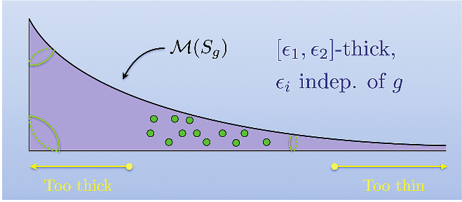
As above, a pseudo-Anosov $f \in \operatorname {MCG}(S)$ corresponds to a loop $\gamma _f \subseteq \mathcal{M}(S)$. We again let $\Psi _L$ denote the set of pseudo-Anosov maps $f$ with $\log \lambda \leq L/g$. With Leininger, we proved the following theorem LM13.

Theorem (Leininger–Margalit).

Given $L$, there exists $\epsilon _1=\epsilon _1(L)$ and $\epsilon _2 = \epsilon _2(L)$ so that

$$\begin{equation*} f \in \Psi _L \Rightarrow \gamma _f \subseteq \mathcal{M}_{[\epsilon _1,\epsilon _2]}(S). \end{equation*}$$

We emphasize that the $\epsilon _i$ are independent of $g$. Our caricature of the theorem is in Figure 15.

Figure 15.

A cartoon of moduli space, with the locations of the small-stretch pseudo-Anosov maps (or, the corresponding loops) indicated by green dots.

Back to Mirzakhani

The set $\Psi _L$ contains subsets $\Psi _{L,g}$ consisting of the small-stretch pseudo-Anosov maps $S_g \to S_g$. In our work with Leininger from the previous section, we obtained a further result: if we fix $L$ and let $g$ vary, the cardinality of $\Psi _{L,g}$ behaves like a polynomial in $g$ (for the precise statements, see Theorems 1.2 and 1.3 in that paper). As mentioned above, the elements of $\Psi _{L,g}$ correspond to the loops of length at most $L$ in $\mathcal{M}(S_g)$. In that sense, this gives a count of short curves in the spirit of Mirzakhani’s theorem about short curves on a surface.

In Mirzakhani’s theorem the variable $g$ is fixed and $L$ varies. And so a more direct analogue of that theorem would be a count of $\Psi _{L,g}$ for fixed $g$ and varying $L$. Fittingly, the more direct analogue was given by Mirzakhani herself, in joint work with her collaborators. Expanding on work of Veech, Eskin and Mirzakhani proved the following EM11.

Theorem (Eskin–Mirzakhani).

For fixed $g$ and varying $L$ the cardinality of $\Psi _{L,g}$ grows exponentially in $L$. In particular it is asymptotic to

$$\begin{equation*} \frac{e^{(6g-6)L}}{(6g-6)L}. \end{equation*}$$

Since $\Psi _{L,g}$ contains all loops in moduli space of length at most $L$, we might think of this theorem as being more analogous to the fact that the number of curves in $S_g$ of length at most $L$ grows exponentially in $L$. With Eskin and Rafi, Mirzakhani proved that the number of loops of length at most $L$ and of a certain topological type (lying in a certain stratum of moduli space) is also exponential in $L$, but with smaller exponent EMR19. This is a striking analogue of Mirzakhani’s theorem about short curves in surfaces.

Epilogue

We study pseudo-Anosov maps with small stretch factor because they are precious stones. They are beautiful in a similar way to the way we think of the golden ratio as being so. This beauty does not come from the decimal expansion of the golden ratio, but from its various, interconnected descriptions in terms of golden rectangles, its algebraic formula $x^2=x+1$, and its continued fraction expansion, to name a few. Like the golden ratio, pseudo-Anosov maps and their stretch factors are gems, wonderful to visualize and contemplate.

Even from the small fragment of her work discussed in this article, we can see that Maryam Mirzakhani’s life’s work is a gem mine. And from the small amount of time I spent with her, I also know that Maryam was a gem of a person, radiating with positive energy, scientific curiosity, and mathematical ideas. Her grace in the most difficult of circumstances fills me with admiration and appreciation. May her memory continue to be a blessing, and may her work continue to be an inspiration for generations to come.