The Symmetric Group Through a Dual Perspective

Mathematicians began the study of representation theory over a hundred years ago. Since then it has become a centerpiece technique in fields such as algebra, topology, number theory, geometry, mathematical physics, quantum information theory, and complexity theory. A premise of representation theory is that we can study groups and algebras from how they act on vector spaces.

In this article we take this a step further; to study actions of a group or algebra we study what commutes with the action. The collection of all linear transformations that commute with the action is called the commutant or the centralizer. The centralizer is itself an algebra which is called the Schur–Weyl dual.

A reason why this has become such an important technique is that it can lead to beautiful connections between seemingly different areas of mathematics. One example of this is the discovery of the Jones polynomial. This polynomial is a one variable invariant for oriented knots or links 67. The polynomial was discovered while studying linear functionals of the Temperley–Lieb algebra, an example of a centralizer algebra. Following this work, Jones received his Fields Medal for discovering deep connections between representation theory, topology, and theoretical physics 7.

In this article we will present how centralizer algebras can be used to study the representation theory of the symmetric group. Although we know a lot about its representation theory, there are still open problems that are out of reach such as the Kronecker problem and the restriction problem that we discuss below. Our approach to these problems has been to use centralizer algebras to develop combinatorial tools to study them.

All of the vector spaces in this article are over the complex numbers $\mathbb{C}$, and $GL_n$ will denote the general linear group of invertible $n\times n$ matrices with complex entries.

What is a representation?

Representation theory is the art of studying abstract algebraic objects, such as groups and algebras, by understanding how they act on vector spaces.

When acting on a vector space, each element in the algebra or group is represented by a linear transformation (or more concretely, a matrix). The set of resulting linear transformations is a representation of the algebra or group. Moreover, multiplying two elements in the algebra or group corresponds to composition of the corresponding linear transformations. It is common to refer to the vector space together with the action as the representation, or if the action is understood to just the vector space as the representation.

In this article we are interested in the representation theory of the symmetric group, $S_k$, the group of bijections from the set $\{1,2, \ldots , k\}$ to itself. There are many ways to represent the elements of $S_k$, in this article we will think of them in cycle notation or as diagrams. For example, $(1,3,4)(5,6)\in S_6$ corresponds to the diagram in Figure 1.

Figure 1.

A diagram depicting the permutation $(1,3,4)(5,6)\in S_6$.

We will use the following example of a representation to illustrate the ideas introduced in this article. Consider

$$\begin{equation*} S_3 = \{e,(1,2),(1,3),(2,3),(1,2,3),(1,3,2)\}, \end{equation*}$$

where $e$ is the identity and the other elements are written using cycle notation (with one-cycles omitted). The symmetric group $S_3$ acts on the vector space $\mathbb{C}^3$. If we choose the basis of standard column vectors for $\mathbb{C}^3$, $\{e_1, e_2, e_3\}$, then an element $\sigma \in S_3$ acts by $\sigma \cdot e_i = e_{\sigma (i)}$. As an example, $(1,2)\cdot e_1 = e_2$, $(1,2)\cdot e_2 = e_1$, and $(1,2)\cdot e_3 = e_3$. Then each $\sigma \in S_3$ is represented by a permutation matrix:

$$\begin{equation*} e \mapsto \left[\begin{array}{ccc} 1 & 0 & 0 \\0& 1 & 0 \\0 & 0 & 1 \end{array} \right], \quad (1,2) \mapsto \left[\begin{array}{ccc} 0 & 1 & 0 \\1 & 0 & 0 \\0 & 0 & 1 \end{array} \right], \end{equation*}$$

$$\begin{equation*} (2,3) \mapsto \left[\begin{array}{ccc} 1 & 0 & 0 \\0& 0 & 1 \\0 & 1 & 0 \end{array} \right], (1,2,3) \mapsto \left[\begin{array}{ccc} 0 & 0 & 1 \\1 & 0 & 0 \\0 & 1 & 0 \end{array} \right], \end{equation*}$$

$$\begin{equation*} (1,3) \mapsto \left[\begin{array}{ccc} 0 & 0 & 1 \\0& 1 & 0 \\1 & 0 & 0 \end{array} \right], (1,3,2) \mapsto \left[\begin{array}{ccc} 0 & 1 & 0 \\0& 0 & 1 \\1 & 0 & 0 \end{array} \right]. \end{equation*}$$

We will refer to this representation as the permutation representation of $S_3$.

To define a representation, we need a vector space and an action of the group or algebra on the vector space. Another way to think of a representation is as a group homomorphism to the general linear group, $GL_n$. For example, the permutation representation of $S_3$ is the homomorphism $\rho : S_3\rightarrow GL_3$ shown above.

Each finite group or finite-dimensional algebra has an infinite number of matrix representations, but we only need a finite number of them to express all of the representations. A common theme in mathematics is to identify the basic building blocks in the theory. For example, in number theory the building blocks are the primes. Applying this idea to representation theory leads to the concept of an irreducible representation, which is a representation that does not contain a subspace that is closed under the action. For instance the permutation representation mentioned above has a subspace $W = {\mathrm{span}}\{ e_1 + e_2 + e_3 \}$ which is closed under the action and hence the permutation representation is not irreducible. The subspace $W$ is an irreducible representation of $S_3$.

In this article, we will restrict our attention to semisimple representations. Just as composite numbers can be written using primes, semisimple representations can be decomposed into direct sums of irreducible ones. Many open problems in combinatorial representation theory ask for algorithms for decomposing representations into irreducible ones.

Representations of the symmetric group

A nontrivial and beautiful fact is that the irreducible representations of a finite group are in bijection with the conjugacy classes of that group. In the case of the symmetric group, $S_n$, the conjugacy classes are determined by cycle type (the lengths of the cycles in cycle notation). Since the cycle type is a partition of $n$, then the irreducible representations are also indexed by these.

Recall that a partition of $n$ is a weakly decreasing sequence $\lambda = (\lambda _1, \lambda _2, \ldots , \lambda _{\ell })$ of nonnegative integers that add up to $n$. We use $|\lambda |$ for the sum $\lambda _1+\lambda _2+ \cdots + \lambda _\ell$. We will think of a partition as a Young diagram, an array of boxes with $\lambda _i$ boxes in the $i$-th row that are left-justified. We will use the English convention in which we write the boxes corresponding to $\lambda _1$ in the top row, $\lambda _2$ in the second row, and so on.

For instance, $S_3$ has three irreducible representations, which are indexed by partitions of 3,

$$\begin{align*} (3) & \rightarrow \vcenter{\img[][27pt][10pt][{\renewcommand{\arraystretch}{1} \setlength{\unitlength}{1.0pt} \begin{tikzpicture}[scale=0.30,every node/.style={font=\rm\small}]\tikztableauinternal{{ \ ,\ ,\ }}\end{tikzpicture}}]{Images/imgbae23b9812ed18fe749b4a7d473e9672.svg}} \ ,\\ (2,1) & \rightarrow \vcenter{\img[][19pt][18pt][{\renewcommand{\arraystretch}{1} \setlength{\unitlength}{1.0pt} \begin{tikzpicture}[scale=0.30,every node/.style={font=\rm\small}]\tikztableauinternal{{ \ ,\ }, {\ }}\end{tikzpicture}}]{Images/imgf047a40070ca9465e4fb8e7c850e8a67.svg}} \ , \\ \text{and} \quad (1,1,1) &\rightarrow \vcenter{\img[][9pt][27pt][{\renewcommand{\arraystretch}{1} \setlength{\unitlength}{1.0pt} \begin{tikzpicture}[scale=0.30,every node/.style={font=\rm\small}]\tikztableauinternal{{ \ },{\ },{\ }}\end{tikzpicture}}]{Images/img3cc5908048738390c848255e9bb36963.svg}}. \end{align*}$$

We use $\mathbb{S}^\lambda$ to denote the irreducible representation indexed by $\lambda$. One way to describe $\mathbb{S}^\lambda$ is by giving a basis and the action of $S_n$ on this basis. Every representation of $S_n$ can be written as a direct sum of irreducible ones. This fact is known as Maschke’s theorem and is a property that is true for representations of finite groups. For example, the permutation representation of $S_3$ is isomorphic ($\cong$) to the direct sum of two irreducible representations, namely

$$\begin{equation*} \mathbb{C}^3 \cong \mathbb{S}^{(2,1)} \oplus \mathbb{S}^{(3)}, \end{equation*}$$

where $\mathbb{S}^{(2,1)} \cong {\mathrm{span}}\{ e_3 - e_1, e_2 - e_1 \}$ and $\mathbb{S}^{(3)} \cong {\mathrm{span}}\{ e_1 + e_2 + e_3 \}$.

Character tables

One of the downsides of thinking about representations in terms of matrices is that the matrices depend on the basis chosen for the vector space. Changing basis produces an isomorphic representation. Fortunately, for complex representations the representations are determined up to isomorphism by their character. The character of a representation $\rho : G\rightarrow GL_d$ is the function $\chi ^\rho : G\rightarrow \mathbb{C}$ defined by

$$\begin{equation*} \chi ^\rho (g) = trace(\rho (g)), \quad \text{for every } g\in G. \end{equation*}$$

Recall that in linear algebra the trace of a matrix is the sum of its diagonal entries. Using properties of the trace function, we can show that two conjugate elements have the same trace and that isomorphic representations have the same character. Therefore, the essence of the representation of a group can be stored in a vector with entries equal to the trace at a representative of a conjugacy class.

For example, the permutation representation of $S_3$ has $\chi ^\rho (e) = 3$,

$$\begin{equation*} \chi ^\rho ((2,1)) = \chi ^\rho ((1,3)) = \chi ^\rho ((2,3))= 1, \end{equation*}$$

$$\begin{equation*} \chi ^\rho ((1,2,3))=\chi ^\rho ((1,3,2)) = 0. \end{equation*}$$ Therefore, we can think of its character as the vector $\chi ^\rho = \langle 3,1,0\rangle$ with one value for each conjugacy class.

The irreducible complex characters of a finite group can be stored compactly in a square matrix where each row corresponds to an irreducible representation and each column corresponds to a conjugacy class, often indexed by a conjugacy class representative. For instance, the character table of $S_3$ is given in Figure 2.

Figure 2.

The irreducible character table for the symmetric group $S_3$.

$$\begin{equation*} \begin{array}{l|c|c|c} & e & (1,2) & (1,2,3)\\\hline \chi ^{(1,1,1)} & 1 & -1 & 1 \\\hline \chi ^{(2,1)} & 2 & 0 & -1 \\\hline \chi ^{(3)} & 1 & 1 & 1 \end{array} \end{equation*}$$

Writing a representation as a direct sum of irreducibles is the same as writing a character as a vector sum of irreducible characters. In our running example, the character of the permutation representation is the sum of two irreducible characters,

$$\begin{equation*} \chi ^\rho = \chi ^{(2,1)} + \chi ^{(3)} = \langle 2,0,-1\rangle + \langle 1, 1, 1\rangle = \langle 3,1,0\rangle . \end{equation*}$$

Characters contain all essential information about representations; in fact, Frobenius developed the representation theory of finite groups completely in terms of their characters.

The Kronecker product

The tensor product of two representations for any group is also a representation. In the special case of the symmetric group, given two irreducible representations, $\mathbb{S}^\lambda$ and $\mathbb{S}^\mu$ with $\lambda$ and $\mu$ both partitions of $n$, $\mathbb{S}^\lambda \otimes \mathbb{S}^\mu$ has underlying vector space the tensor product of the vectors spaces for $\mathbb{S}^\lambda$ and $\mathbb{S}^\mu$. If $v\otimes w\in \mathbb{S}^\lambda \otimes \mathbb{S}^\mu$, then $\sigma \in S_n$ acts diagonally, i.e., $\sigma \cdot v\otimes w = \sigma \cdot v \otimes \sigma \cdot w$.

The character of $\mathbb{S}^\lambda \otimes \mathbb{S}^\mu$, written $\chi ^{\lambda \otimes \mu }$, is the point-wise product of the characters of $\mathbb{S}^\lambda$ and $\mathbb{S}^\mu$, i.e., for $g\in S_n$,

$$\begin{equation*} \chi ^{\lambda \otimes \mu }(g) = \chi ^\lambda (g) \chi ^\mu (g). \end{equation*}$$

For example, using character vectors with $\lambda = \mu = (2,1)$ (see the character table for $S_3$)

$$\begin{equation*} \chi ^{(2,1)\otimes (2,1)} = \langle 2,0, -1\rangle \langle 2,0,-1\rangle = \langle 4, 0, 1\rangle . \end{equation*}$$

An interesting challenge is to write a tensor product such as $\chi ^{(2,1) \otimes (2,1)}$ as a sum of irreducible characters. In this case, by playing around with the character table in Figure 2, we can see that

$$\begin{equation*} \chi ^{(2,1)\otimes (2,1)} = \chi ^{(3)} +\chi ^{(2,1)} + \chi ^{(1,1,1)}. \end{equation*}$$

In general, the coefficients of the irreducible characters, $g(\lambda ,\mu ,\nu )$, are the nonnegative integers which describe the number of times that the irreducible character $\chi ^\nu$ occurs in the decomposition of $\chi ^{\lambda \otimes \mu }$ when written as a sum of irreducibles,

$$\begin{equation*} \chi ^{\lambda \otimes \mu } = \sum _\nu g(\lambda ,\mu ,\nu ) \chi ^\nu . \end{equation*}$$

In combinatorial representation theory we are interested in finding combinatorial algorithms to compute the coefficients and tie them to enumerable set of objects. Then, we use this set to deduce properties of the coefficients. The following is a well-known open problem in this area:

The Kronecker problem

Find a set of objects depending only on $\lambda$, $\mu$, and $\nu$ with cardinality $g(\lambda ,\mu ,\nu )$. We call this a combinatorial interpretation.

This problem has motivated decades of research since the early 1900s. Most recently this is due to deep connections with quantum information theory 3 and the central role it plays within Geometric Complexity Theory 11. This is an approach that seeks to settle the celebrated P versus NP problem, one of the several Millennium Prize Problems set by the Clay Mathematics Institute.

Why a combinatorial interpretation?

Combinatorial interpretations of the multiplicities often lead to the discovery of new properties, a better understanding, and in some cases to proofs of longstanding open problems. For example, Knutson and Tao found a combinatorial model for the multiplicities occurring in the tensor product of representations of the general linear group. They used their model to prove the saturation property of these coefficients and this led to a proof of Horn’s conjecture from 1962 characterizing the spectrum of the sum of two Hermitian matrices 9.

Stability of Kronecker coefficients

The Kronecker product of symmetric group representations satisfies a stability property first discovered by Murnaghan 212. Murnaghan observed that for sufficiently large $n$, the decomposition of $\chi ^{(n - |\alpha |, \alpha )\otimes (n -|\beta |,\beta )}$ only depends on the parts of $\alpha$ and $\beta$ and not on $n$. For example, for $n\geq 7$, we always get the following decomposition when $\alpha =(1)$ and $\beta =(2,1)$:

$$\begin{align*} \chi ^{(n-1,1)\otimes (n-3,2,1)} = & \, \chi ^{(n-2,1, 1)} + \chi ^{(n-3,1, 1, 1)} \\ & +\chi ^{(n-2,2)} + 2\chi ^{(n-3,2, 1)} \\ & +\chi ^{(n-3,3)}+\chi ^{(n-4,2, 1, 1)} \\ & + \chi ^{(n-4,2, 2)}+ \chi ^{(n-4,3, 1)}. \end{align*}$$

In general, we get nonnegative integer coefficients, $\overline{g}_{\alpha ,\beta }^\gamma$ that depend on three partitions $\alpha$, $\beta$, and $\gamma$. These coefficients are called reduced (or stable) Kronecker coefficients.

A duality between $S_k$ and $GL_n$

In general, a representation of $GL_n$ is a homomorphism, $\rho : GL_n \rightarrow GL_d$. However, the representation theory of $GL_n$ can get pretty wild. In algebraic combinatorics, we often restrict our attention to polynomial representations. This means that the matrices $\rho (A)$ have polynomial entries in the entries of the matrix $A\in GL_n$. The irreducible polynomial representations are indexed by partitions with at most $n$ parts. The polynomial representations of $GL_n$ were first studied by Issai Schur in his 1901 thesis under the supervision of Frobenius.

By fixing a basis of a three-dimensional vector space, an example of a polynomial representation $\rho : GL_2\rightarrow GL_3$ is given by the following matrix:

$$\begin{equation*} \rho \left(\left[\begin{array}{cc} a & b \\c & d \end{array} \right]\right) = \left[ \begin{array}{ccc} a^2 & 2ab & b^2 \\ac & ad+bc & bd \\c^2 & 2cd & d^2 \end{array}\right]. \end{equation*}$$

In 1927, Schur reformulated his thesis results in what today is known as the Schur–Weyl duality. This duality defines a correspondence between irreducible representations of the symmetric group $S_k$ and irreducible, homogeneous, polynomial representations of $GL_n$ of degree $k$. Letting $V = \mathbb{C}^n$, $GL_n$ acts diagonally on $V^{\otimes k}$ ($k$-fold tensor product of $V$), that is, for $A\in GL_n$ and $v_1\otimes \cdots \otimes v_k$ in $V^{\otimes k}$,

$$\begin{equation*} A\cdot (v_1\otimes v_2\otimes \cdots \otimes v_k) = Av_1\otimes Av_2\otimes \cdots \otimes Av_k. \end{equation*}$$

Concretely, $Av_i$ is the product of the matrix $A$ with the column vector $v_i$. The symmetric group $S_k$ also has a right action of $V^{\otimes k}$ by permuting the tensor factors. For example, for $\sigma = (1,3,4)\in S_4$, $v_a\otimes v_b\otimes v_c\otimes v_d\cdot (1,3,4) = v_d\otimes v_b\otimes v_a\otimes v_c$, where $1\leq a,b,c,d\leq n$, which can be visualized in Figure 3.

Figure 3.

Visualization of the right action of $(1,3,4)$ in $S_4$ on a tensor in $V^{\otimes 4}$.

The basic observation that Schur made is that the diagonal action of $GL_n$ and the permutation action of $S_k$ commute. This implies there is a well-defined action of the group $GL_n \times S_k$ (direct product) on $V^{\otimes k}$. When we decompose $V^{\otimes k}$ in terms of irreducible representations of $GL_n\times S_k$ we get

$$\begin{equation} V^{\otimes k} \cong \bigoplus _\lambda \mathbb{V}^\lambda \otimes \mathbb{S}^\lambda , {\tag{1}} \end{equation}$$

where $\mathbb{V}^\lambda$ is an irreducible, homogeneous, polynomial representation of $GL_n$ and $\lambda$ runs over all partitions of $k$ with at most $n$ parts. This gives a correspondence between representations of $S_k$ and polynomial representations of $GL_n$.

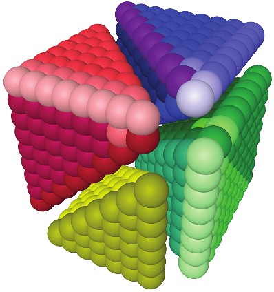
Consider the case when $k=3$ and $n=9$. Combinatorics can help to visualize $V^{\otimes 3}$ and how it decomposes following Equation 1. Figure 4 represents basis elements of $V^{\otimes 3}$ as $(i_1, i_2, i_3)$ in three-dimensional space with $1 \leq i_1, i_2, i_3 \leq 9$ and organizes them so that the irreducible $GL_9$ components are compact. The blue points represent $\mathbb{V}^{(3)} \otimes \mathbb{S}^{(3)}$, the red and the green points together represent $\mathbb{V}^{(2,1)} \otimes \mathbb{S}^{(2,1)}$ and the yellow points represent $\mathbb{V}^{(1,1,1)} \otimes \mathbb{S}^{(1,1,1)}$. The Robinson–Schensted algorithm 16 gives a way of making this assignment in general.

Figure 4.

A combinatorial view of the decomposition of $V^{\otimes 3}$ into $GL_9$ representations.

Characters of $GL_n$

A polynomial in commuting variables $x_1, \ldots , x_n$ is symmetric if any permutation of the variables leaves the polynomial invariant. For every polynomial representation of $GL_n$, there exists a symmetric polynomial $f(x_1, \ldots , x_n)$ such that if $A \in GL_n$ has eigenvalues $\theta _1, \ldots , \theta _n$, then the character value at $A$ is $f(\theta _1, \ldots , \theta _n)$. In the previous section we saw that for every partition $\lambda$ with at most $n$ parts, there exists an irreducible polynomial representation of $GL_n$ which we refer to as ${\mathbb{V}}^\lambda$. Schur showed the character corresponding to ${\mathbb{V}}^\lambda$ are obtained by evaluations of a polynomial $s_{\lambda }(x_1, \ldots , x_n)$ which is constructed combinatorially as follows:

1.

In the boxes of the Young diagram of $\lambda$ insert numbers $1,2,\ldots , n$ so that the numbers increase weakly along each row from left to right and strictly from top to bottom in each column. This is called a semistandard Young tableau (SSYT for short).

For example, if $\lambda = (2)$ then its Young diagram is ${\vcenter{\img[][19pt][10pt][{\renewcommand{\arraystretch}{1} \setlength{\unitlength}{1.0pt} \begin{tikzpicture}[scale=0.30,every node/.style={font=\rm\small}]\tikztableauinternal{{ , }}\end{tikzpicture}}]{Images/img2ddfb67edc408c683f83a9ab6dd1a541.svg}}}$. If $n=3$, these are the possible tableaux:$$\begin{equation*} \vcenter{\img[][19pt][10pt][{\renewcommand{\arraystretch}{1} \setlength{\unitlength}{1.0pt} \begin{tikzpicture}[scale=0.30,every node/.style={font=\rm\small}]\tikztableauinternal{{1 ,1 }}\end{tikzpicture}}]{Images/img6b169a7fbde5fe4af3dcf990c1d40e01.svg}},\ \vcenter{\img[][19pt][10pt][{\renewcommand{\arraystretch}{1} \setlength{\unitlength}{1.0pt} \begin{tikzpicture}[scale=0.30,every node/.style={font=\rm\small}]\tikztableauinternal{{1 ,2}}\end{tikzpicture}}]{Images/img578e21f8fc8c8ed7f6188ac7a4194b40.svg}},\ \vcenter{\img[][19pt][10pt][{\renewcommand{\arraystretch}{1} \setlength{\unitlength}{1.0pt} \begin{tikzpicture}[scale=0.30,every node/.style={font=\rm\small}]\tikztableauinternal{{1 ,3}}\end{tikzpicture}}]{Images/imgea798ca4c53f7907a32035b6da30dfd9.svg}},\ \vcenter{\img[][19pt][10pt][{\renewcommand{\arraystretch}{1} \setlength{\unitlength}{1.0pt} \begin{tikzpicture}[scale=0.30,every node/.style={font=\rm\small}]\tikztableauinternal{{ 2 ,2 }}\end{tikzpicture}}]{Images/img12b81bc45d9dfce79330cd45bdc42b44.svg}}, \ \vcenter{\img[][19pt][10pt][{\renewcommand{\arraystretch}{1} \setlength{\unitlength}{1.0pt} \begin{tikzpicture}[scale=0.30,every node/.style={font=\rm\small}]\tikztableauinternal{{ 2 ,3 }}\end{tikzpicture}}]{Images/imge3a8354e33cc876c539bfcd07a96772b.svg}},\ \vcenter{\img[][19pt][10pt][{\renewcommand{\arraystretch}{1} \setlength{\unitlength}{1.0pt} \begin{tikzpicture}[scale=0.30,every node/.style={font=\rm\small}]\tikztableauinternal{{ 3 ,3 }}\end{tikzpicture}}]{Images/imgfcc674e0a6811a8c7134cad2be88da15.svg}}. \end{equation*}$$

2.

For each tableau, $T$, in part (1), define a monomial $x^T = x_1^{i_1}x_2^{i_2}\cdots x_n^{i_n}$, where $i_j$ is the number of times that $j$ occurs in $T$. For example, the corresponding monomials for the SSYT above are $x_1^2$, $x_1x_2$, $x_1x_3$, $x_2^2$, $x_2x_3$, and $x_3^2$, respectively.

3.

The Schur polynomial $s_{\lambda }(x_1, \ldots , x_n)$ is defined by summing all monomials possible:$$\begin{equation*} s_{\lambda }(x_1, \ldots , x_n) = \sum _{T} x^T, \end{equation*}$$

where the sum is over all SSYT constructed using $\lambda$ and $1,2,\ldots n$.

In the case of our running example, we get

$$\begin{equation*} s_{(2)}(x_1,x_2,x_3) = x_1^2 + x_1x_2 + x_1x_3+x_2^2+x_2x_3+x_3^2. \end{equation*}$$

The interested reader may check that the polynomial is symmetric since permuting the indices $1$, $2$, and $3$ in any way gives the same polynomial. In addition one may verify by listing the tableaux of shape $(1,1)$ that

$$\begin{equation*} s_{(1,1)}(x_1,x_2,x_3) = x_1x_2+ x_1x_3+x_2x_3. \end{equation*}$$

If $A\in GL_n$ has eigenvalues $\theta _1, \ldots , \theta _n$, then the character value for the representation $\mathbb{V}^\lambda$ when acted on by $A$ is obtained by substituting $x_i = \theta _i$, for all $i$, in $s_\lambda (x_1, \ldots , x_n)$. The number $s_\lambda (\theta _1, \ldots , \theta _n)$ is the trace of the matrix representing $A$ when $A$ acts on a basis of $\mathbb{V}^\lambda$. For example, if $A$ has eigenvalues $1, -1,$ and $2$, then setting $x_1 =1$, $x_2 = -1$, and $x_3 =2$ in $s_{(2)}(x_1, x_2, x_3)$ gives the character of the representation $\mathbb{V}^{(2)}$ of $GL_3$ at the matrix $A$. In this case, $s_{(2)} (1, -1, 2) = 5$ is the character value.

Restricting representations

Any polynomial representation of $GL_n$ is a representation for any subgroup $G$ of $GL_n$. In particular, the symmetric group $S_n$, thought of as the group of $n \times n$ permutation matrices, is a subgroup of $GL_n$. Therefore, for any $\lambda$, $\mathbb{V}^\lambda$ is a representation of $S_n$. We write $\text{Res}_{S_n}\mathbb{V}^\lambda$ for this restricted representation. The following is a well-known open problem, for more details and references see 13.

The Restriction Problem: Given an irreducible polynomial representation of $GL_n$, $\mathbb{V}^\lambda$, give a combinatorial algorithm to compute the coefficients, $r_{\lambda ,\mu }$, that occur when restricted to the symmetric group in the equation

$$\begin{equation*} Res_{S_n} \mathbb{V}^\lambda \cong \bigoplus _\mu r_{\lambda ,\mu } \mathbb{S}^\mu . \end{equation*}$$

We can obtain the character of the restricted representation $Res_{S_n} \mathbb{V}^\lambda$ by evaluating $s_\lambda (x_1, x_2,\ldots , x_n)$ only at eigenvalues of permutation matrices.

For example, if $n=3$ we can restrict $\mathbb{V}^{(2)}$ with character

$$\begin{equation*} s_{(2)}(x_1,x_2,x_3) = x_1^2 + x_1x_2 + x_1x_3+x_2^2+x_2x_3+x_3^2 \end{equation*}$$

to $S_3$. To get the character, for each conjugacy class of $S_3$ choose a representative and compute its eigenvalues. The identity, $e$, has eigenvalues $1, 1, 1$, a two-cycle has eigenvalues $1, 1, -1$, and $1, \xi , \xi ^2$ are the eigenvalues for a three-cycle, where $\xi$ is a primitive third root of unity. Then evaluate, $s_{(2)}(1,1,1) = 6$, $s_{(2)}(1,1,-1) = 2$, and $s_{(2)}(1,\xi ,\xi ^2) =0$. Thus, again using the character table in Figure 2, the character of $\text{Res}_{S_3}\mathbb{V}^{(2)}$ is the vector $\langle 6, 2,0\rangle = 2\ \chi ^{(3)} + 2 \ \chi ^{(2,1)}$. We can see that $r_{(2),(3)} =2$ and $r_{(2),(2,1)} = 2$.

Figure 5.

A combinatorial view of the decomposition of $V^{\otimes 3}$ into $GL_9$ representations by primary colors and then the restriction of those into $S_9$ representations by the different shades of those regions.

A dual approach to restriction

Schur used the diagonal action of $GL_n$ on

References

- [1]
- C. Bowman, M. De Visscher, and R. Orellana, The partition algebra and the Kronecker coefficients, Trans. Amer. Math. Soc. 367 (2015), no. 5, 3647–3667, DOI 10.1090/S0002-9947-2014-06245-4. MR3314819,
Show rawAMSref
\bib{BDO}{article}{ author={Bowman, C.}, author={De Visscher, M.}, author={Orellana, R.}, title={The partition algebra and the Kronecker coefficients}, journal={Trans. Amer. Math. Soc.}, volume={367}, date={2015}, number={5}, pages={3647--3667}, issn={0002-9947}, review={\MR {3314819}}, doi={10.1090/S0002-9947-2014-06245-4}, } - [2]
- Emmanuel Briand, Rosa Orellana, and Mercedes Rosas, The stability of the Kronecker product of Schur functions, J. Algebra 331 (2011), 11–27, DOI 10.1016/j.jalgebra.2010.12.026. MR2774644,
\bib{BOR}{article}{ author={Briand, Emmanuel}, author={Orellana, Rosa}, author={Rosas, Mercedes}, title={The stability of the Kronecker product of Schur functions}, journal={J. Algebra}, volume={331}, date={2011}, pages={11--27}, issn={0021-8693}, review={\MR {2774644}}, doi={10.1016/j.jalgebra.2010.12.026}, } - [3]
- Matthias Christandl, Aram W. Harrow, and Graeme Mitchison, Nonzero Kronecker coefficients and what they tell us about spectra, Comm. Math. Phys. 270 (2007), no. 3, 575–585, DOI 10.1007/s00220-006-0157-3. MR2276458,
\bib{CHG}{article}{ author={Christandl, Matthias}, author={Harrow, Aram W.}, author={Mitchison, Graeme}, title={Nonzero Kronecker coefficients and what they tell us about spectra}, journal={Comm. Math. Phys.}, volume={270}, date={2007}, number={3}, pages={575--585}, issn={0010-3616}, review={\MR {2276458}}, doi={10.1007/s00220-006-0157-3}, } - [4]
- Tom Halverson, Characters of the partition algebras, J. Algebra 238 (2001), no. 2, 502–533, DOI 10.1006/jabr.2000.8613. MR1823772,
\bib{halverson}{article}{ author={Halverson, Tom}, title={Characters of the partition algebras}, journal={J. Algebra}, volume={238}, date={2001}, number={2}, pages={502--533}, issn={0021-8693}, review={\MR {1823772}}, doi={10.1006/jabr.2000.8613}, } - [5]
- Tom Halverson and Arun Ram, Partition algebras, European J. Combin. 26 (2005), no. 6, 869–921, DOI 10.1016/j.ejc.2004.06.005. MR2143201,
\bib{halversonram}{article}{ author={Halverson, Tom}, author={Ram, Arun}, title={Partition algebras}, journal={European J. Combin.}, volume={26}, date={2005}, number={6}, pages={869--921}, issn={0195-6698}, review={\MR {2143201}}, doi={10.1016/j.ejc.2004.06.005}, } - [6]
- Vaughan F. R. Jones, A polynomial invariant for knots via von Neumann algebras, Bull. Amer. Math. Soc. (N.S.) 12 (1985), no. 1, 103–111, DOI 10.1090/S0273-0979-1985-15304-2. MR766964,
\bib{jones1}{article}{ author={Jones, Vaughan F. R.}, title={A polynomial invariant for knots via von Neumann algebras}, journal={Bull. Amer. Math. Soc. (N.S.)}, volume={12}, date={1985}, number={1}, pages={103--111}, issn={0273-0979}, review={\MR {766964}}, doi={10.1090/S0273-0979-1985-15304-2}, } - [7]
- V. F. R. Jones, Hecke algebra representations of braid groups and link polynomials, Ann. of Math. (2) 126 (1987), no. 2, 335–388, DOI 10.2307/1971403. MR908150,
\bib{jones2}{article}{ author={Jones, V. F. R.}, title={Hecke algebra representations of braid groups and link polynomials}, journal={Ann. of Math. (2)}, volume={126}, date={1987}, number={2}, pages={335--388}, issn={0003-486X}, review={\MR {908150}}, doi={10.2307/1971403}, } - [8]
- V. F. R. Jones, The Potts model and the symmetric group, Subfactors (Kyuzeso, 1993), World Sci. Publ., River Edge, NJ, 1994, pp. 259–267. MR1317365,
\bib{jones3}{article}{ author={Jones, V. F. R.}, title={The Potts model and the symmetric group}, conference={ title={Subfactors}, address={Kyuzeso}, date={1993}, }, book={ publisher={World Sci. Publ., River Edge, NJ}, }, date={1994}, pages={259--267}, review={\MR {1317365}}, } - [9]
- Allen Knutson and Terence Tao, The honeycomb model of tensor products. I. Proof of the saturation conjecture, J. Amer. Math. Soc. 12 (1999), no. 4, 1055–1090, DOI 10.1090/S0894-0347-99-00299-4. MR1671451,
\bib{knutson-tao}{article}{ author={Knutson, Allen}, author={Tao, Terence}, title={The honeycomb model of $\mathrm {GL}_n(\mathbf {C})$ tensor products. I. Proof of the saturation conjecture}, journal={J. Amer. Math. Soc.}, volume={12}, date={1999}, number={4}, pages={1055--1090}, issn={0894-0347}, review={\MR {1671451}}, doi={10.1090/S0894-0347-99-00299-4}, } - [10]
- Paul Martin, Temperley-Lieb algebras for nonplanar statistical mechanics—the partition algebra construction, J. Knot Theory Ramifications 3 (1994), no. 1, 51–82, DOI 10.1142/S0218216594000071. MR1265453,
\bib{martin}{article}{ author={Martin, Paul}, title={Temperley-Lieb algebras for nonplanar statistical mechanics---the partition algebra construction}, journal={J. Knot Theory Ramifications}, volume={3}, date={1994}, number={1}, pages={51--82}, issn={0218-2165}, review={\MR {1265453}}, doi={10.1142/S0218216594000071}, } - [11]
- Ketan D. Mulmuley and Milind Sohoni, Geometric complexity theory. I. An approach to the P vs. NP and related problems, SIAM J. Comput. 31 (2001), no. 2, 496–526, DOI 10.1137/S009753970038715X. MR1861288,
\bib{MS}{article}{ author={Mulmuley, Ketan D.}, author={Sohoni, Milind}, title={Geometric complexity theory. I. An approach to the P vs. NP and related problems}, journal={SIAM J. Comput.}, volume={31}, date={2001}, number={2}, pages={496--526}, issn={0097-5397}, review={\MR {1861288}}, doi={10.1137/S009753970038715X}, } - [12]
- F. D. Murnaghan, The Analysis of the Kronecker Product of Irreducible Representations of the Symmetric Group, Amer. J. Math. 60 (1938), no. 3, 761–784, DOI 10.2307/2371610. MR1507347,
\bib{murnaghan}{article}{ author={Murnaghan, F. D.}, title={The Analysis of the Kronecker Product of Irreducible Representations of the Symmetric Group}, journal={Amer. J. Math.}, volume={60}, date={1938}, number={3}, pages={761--784}, issn={0002-9327}, review={\MR {1507347}}, doi={10.2307/2371610}, } - [13]
- Rosa Orellana and Mike Zabrocki, Symmetric group characters as symmetric functions, Adv. Math. 390 (2021), Paper No. 107943, 34, DOI 10.1016/j.aim.2021.107943. MR4295089,
\bib{OZ1}{article}{ author={Orellana, Rosa}, author={Zabrocki, Mike}, title={Symmetric group characters as symmetric functions}, journal={Adv. Math.}, volume={390}, date={2021}, pages={Paper No. 107943, 34}, issn={0001-8708}, review={\MR {4295089}}, doi={10.1016/j.aim.2021.107943}, } - [14]
- Rosa Orellana and Mike Zabrocki, The Hopf structure of symmetric group characters as symmetric functions, Algebr. Comb. 4 (2021), no. 3, 551–574, DOI 10.5802/alco.170. MR4275829,
\bib{OZ2}{article}{ author={Orellana, Rosa}, author={Zabrocki, Mike}, title={The Hopf structure of symmetric group characters as symmetric functions}, journal={Algebr. Comb.}, volume={4}, date={2021}, number={3}, pages={551--574}, review={\MR {4275829}}, doi={10.5802/alco.170}, } - [15]
- Rosa Orellana and Mike Zabrocki, Products of symmetric group characters, J. Combin. Theory Ser. A 165 (2019), 299–324, DOI 10.1016/j.jcta.2019.02.019. MR3944530,
\bib{OZ3}{article}{ author={Orellana, Rosa}, author={Zabrocki, Mike}, title={Products of symmetric group characters}, journal={J. Combin. Theory Ser. A}, volume={165}, date={2019}, pages={299--324}, issn={0097-3165}, review={\MR {3944530}}, doi={10.1016/j.jcta.2019.02.019}, } - [16]
- Bruce E. Sagan, The symmetric group, The Wadsworth & Brooks/Cole Mathematics Series, Wadsworth & Brooks/Cole Advanced Books & Software, Pacific Grove, CA, 1991. Representations, combinatorial algorithms, and symmetric functions. MR1093239,
\bib{sagan}{book}{ author={Sagan, Bruce E.}, title={The symmetric group}, series={The Wadsworth \& Brooks/Cole Mathematics Series}, note={Representations, combinatorial algorithms, and symmetric functions}, publisher={Wadsworth \& Brooks/Cole Advanced Books \& Software, Pacific Grove, CA}, date={1991}, pages={xviii+197}, isbn={0-534-15540-5}, review={\MR {1093239}}, } - [17]
- Richard P. Stanley, Enumerative combinatorics. Vol. 2, Cambridge Studies in Advanced Mathematics, vol. 62, Cambridge University Press, Cambridge, 1999. With a foreword by Gian-Carlo Rota and appendix 1 by Sergey Fomin, DOI 10.1017/CBO9780511609589. MR1676282,
\bib{stanley}{book}{
author={Stanley, Richard P.},
title={Enumerative combinatorics. Vol. 2},
series={Cambridge Studies in Advanced Mathematics},
volume={62},
note={With a foreword by Gian-Carlo Rota and appendix 1 by Sergey Fomin},
publisher={Cambridge University Press, Cambridge},
date={1999},
pages={xii+581},
isbn={0-521-56069-1},
isbn={0-521-78987-7},
review={\MR {1676282}},
doi={10.1017/CBO9780511609589},
}
Rosa Orellana is a professor of mathematics at Dartmouth College. Her email address is Rosa.C.Orellana@dartmouth.edu.
Mike Zabrocki is a professor of mathematics at York University. His email address is zabrocki@yorku.ca.
Article DOI: 10.1090/noti2704
Credits
All article images are courtesy of Rosa Orellana and Mike Zabrocki.
Photo of Rosa Orellana is courtesy of Gael Popescu.
Photo of Mike Zabrocki is courtesy of Mike Zabrocki.