Tropical Geometry Forwards and Backwards

Tropical geometry is a relatively recent network of ideas at the intersection of geometry and combinatorics. In its purest form, tropical geometry is a combinatorial analogue of algebraic geometry and can be studied logically independently from it. The basic objects in tropical geometry are things like graphs or simplicial complexes. They are decorated with some additional data that allows them to coarsely mimic objects from algebraic geometry. The properties of these objects are constrained by combinatorial analogues of the basic theorems in geometry. For example, the tropical analogue of a Riemann surface is a graph, and there are purely combinatorial analogues of the Riemann–Roch and Riemann–Hurwitz theorems for graphs. The surprising turn is often that theorem statements in tropical geometry are the same as or similar to parallel ones in algebraic geometry, even though all the words mean something completely different.

While these tropical objects are very interesting in their own right, tropicalization is a process that turns algebraic varieties into tropical objects. This bridges the two worlds and sets up an intricate and imperfect dictionary: geometric constraints imply combinatorial ones and combinatorial constraints imply geometric ones. An enjoyable and compelling part of the subject is that even when there is not a logical implication, known theorems on each side provide predictions and conjectures for results on the other.

The present article aims to give the reader a feel for this network, some of its subtleties, and how it is used. The first topic is a quick and dirty introduction to the process of tropicalization, and some of the early observations in the subject that might have inspired people to look closer. The next topic is the “backwards direction,” i.e., the tropical inverse problem. Our main goal here will be to exhibit one interesting example of a non-realizable tropical object, and give some sense for why it is non-realizable. Finally, we sketch how tropicalization, both forwards and backwards, predicts new theorems in traditional algebraic geometry.

The prototypical tropicalization

The simplest example of tropicalization applies to spaces defined by algebraic equations inside the algebraic torus, i.e., $(\mathbb{C}^\star )^n$. We start with a collection of Laurent polynomials $f_1,\ldots , f_k$ in $n$ variables and look at their common zeroes:

$$\begin{equation*} V = \{f_1 = f_2 = \cdots = f_k = 0\}\subset (\mathbb{C}^\star )^n. \end{equation*}$$

Objects $V$ that are defined in this fashion are the local building blocks in algebraic geometry. They are examples of algebraic varieties. The primary move in tropical geometry comes from the map:

$$\begin{align*} \mathrm{Log}_t: (\mathbb{C}^\star )^n&\to \mathbb{R}^n,\\ (z_1,\ldots ,z_n)&\mapsto (\log _t|z_1|,\ldots ,\log _t|z_n|), \end{align*}$$

where the logarithm has base $t$, some real number. The right-hand side tracks the logarithmic size of a tuple of complex numbers. The image of $V$ under this map, namely $\mathrm{Log}_t(V)$, is the set of possible sizes of solutions to the equations $\{f_i\}$. The motivation behind this move is to split the process of studying solutions to polynomial systems into two steps: first study the possible sizes of solutions and then study solutions of a fixed size.

It is useful to slightly repackage the information. By the logarithm rules, if $t$ changes the set $\mathrm{Log}_t(V)$ is rescaled. The tropicalization is the limit of this rescaling as the base becomes small:

$$\begin{equation*} \mathrm{trop}(V) = \lim _{t\to 0}\mathrm{Log}_t(V). \end{equation*}$$

The limit procedure reveals a simple combinatorial structure. We will see some examples soon, but for now, let us note that this process is a completely elementary but strange thing to do to an algebro-geometric object. At first sight, the nice structure that $V$ inherits from being defined by polynomials might be destroyed by applying this transcendental “limit logarithm” operation. A fundamental theorem of Bieri and Groves from the 1980s reveals that $\mathrm{trop}(V)$ is far from chaotic.

Theorem 0.0.1.

Let $V\subset (\mathbb{C}^\star )^n$ be an algebraic variety of dimension $r$. Then the tropicalization $\mathrm{trop}(V)$ is a polyhedral complex of dimension $r$ in $\mathbb{R}^n$.

Polyhedral complexes are very concrete structures, analogous to the simplicial complexes that one encounters in topology. Just as simplicial complexes are glued from simplices, polyhedral complexes are glued from (a finite number of) polyhedra. A polyhedron in $\mathbb{R}^n$ is any locus where a fixed finite collection of affine functions is non-negative. Examples of this include the familiar polytopes in $\mathbb{R}^2$, as well as unbounded regions such as $\mathbb{R}^m_{\geq 0}$. We will see a few examples below, and reader will be able to find precise definitions and numerous pictures and examples in the textbook 10.

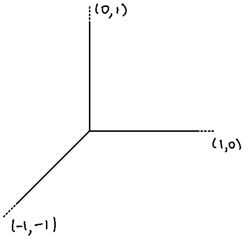
The first entry in almost everyone’s database of tropicalizations is depicted in the figure below. It shows the tropicalization of the curve $\{x+y+1 = 0\}$ in $(\mathbb{C}^\star )^2$. The tropicalization is a union of three rays (which are simple examples of polyhedra), based at the origin, in $\mathbb{R}^2$. There is one ray each in the direction of the positive $x$-axis, positive $y$-axis, and the negative diagonal direction. The picture can be obtained by an explicit calculation, but the reader may find it a pleasant exercise to use a computer to plot a large number of points and see the figure emerge.

Figure 1.

The tropicalization of the curve $C_1$ given by $\{x+y+1=0\}$.

Prettier pictures

In the literature, the term tropicalization is used for a myriad of different operations, but they are all based on the maneuver above. An important upgrade that will be relevant in our discussion is allowing the equations $f_1,\ldots , f_k$ to depend on the base of the logarithm $t$. Precisely, we can choose each $f_i$ to be a polynomial whose coefficients are polynomials, or even power series, in the variable $t$. For some of the statements later in this article to hold, we should allow the coefficients to at least be a power series in $t$ that converges in some neighborhood of $0$, but I encourage the reader to imagine that the coefficients are polynomials in $t$. When there is a dependence on a parameter $t$, we sometimes refer to this as a family of varieties, imagining that for each value of $t$ there is a different variety.

The generalization to allow variable coefficients leads to much richer pictures, which betters our odds of transporting meaningful information into tropical geometry. Without varying the coefficients, the tropicalization of a cubic could, and likely would, look exactly like the tropicalization of the curve $C_1$ that we discussed above.

For example, let us take $f$ to be a degree-$3$ polynomial in $x$ and $y$. There are $10$ possible coefficients to choose when doing this, as we can write the polynomial as a sum of monomials:

$$\begin{equation*} f(x,y) = \sum a_{ij} x^i y^j. \end{equation*}$$

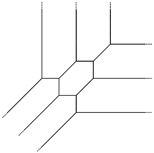
We can now choose the $a_{ij}$ to themselves be polynomials in $t$ and then tropicalize $C_2 = \{f = 0\}$. For example, we could choose the coefficients of each $x^iy^j$ to simply be different powers of $t$. I won’t do out the calculation here, but if these powers of $t$ in front of the monomials $x^iy^j$ are chosen in a sufficiently random way, the tropicalization could look like the picture below. Different choices of coefficients $a_{ij}$ will lead to different pictures, and in fact, there are over 1000 possibilities for tropicalizations of cubics! Nevertheless, the process of going from such polynomials to their tropicalizations is rather concrete, and can be found in the early chapters of the text 10. Despite the numerous possibilities for the actual tropicalization, in most cases, the key features of the picture below will persist.

Figure 2.

The tropicalization of the curve $C_2$ given by the vanishing set of cubic equations, with coefficients depending on a parameter $t$.

A first look at the tropical dictionary

The Bieri–Groves theorem already asserts that the tropicalization of a variety $V$ in $(\mathbb{C}^\star )^n$ sees the dimension of $V$. The calculation of the dimension of algebraic varieties that arise naturally in mathematics has been the content of several deep theorems, so this already has significant potential.

But staring at the pictures, you might start to get a sense that there’s quite a lot more going on here. Let us examine a few suspicious coincidences. First, a little differential topology and analysis tells us what the spaces $C_1$ and $C_2$ look like when they are given their Euclidean topology. It turns out that $C_1$ is homeomorphic to a sphere $\mathbb{S}^2$ minus three points, while, for each small nonzero value of $t$, the space $C_2$ is homeomorphic to the torus $\mathbb{S}^1\times \mathbb{S}^1$ minus $9$ distinct points.

Now let us look at the tropicalizations. Looking at $C_1$, one notices the coincidence of $3$: the legs running off to infinity in $\mathrm{trop}(C_1)$ and the missing points in $C_1$. In the case of $C_2$, one might notice the coincidence of $9$, again between the legs and the missing points. In this case, one might also notice that the topological surface $C_2$ has genus $1$ while $\mathrm{trop}(C_2)$ has a cycle in the middle.

Another interesting coincidence comes from placing $\mathrm{trop}(C_1)$ and $\mathrm{trop}(C_2)$ in the same picture. If the pictures are shifted around a little bit, one can notice that in most cases, the two tropicalizations intersect at exactly three points. But we know that in most cases, $C_1\cap C_2$ is also exactly three points (for each value of the parameter $t$)—if we plug in the equation for $C_2$ into $C_1$ we end up with a cubic in $1$ variable.

Figure 3.

The tropicalizations of a cubic curve and of a line seem to intersect at three points.

If the degree of the polynomial $f$ above was changed from $3$ to $d$, the corresponding curve $\mathbb{V}(f)$ would—if the polynomial was chosen with a little bit of care—have genus $\frac{(d-1)(d-2)}{2}$ and have $3d$ missing points, and sure enough, there would be exactly $\frac{(d-1)(d-2)}{2}$ independent cycles in $\mathrm{trop}(\mathbb{V}(f))$ and exactly $3d$ legs running off to infinity. Now, we’ve certainly not rigorously argued that any of these geometric invariants, such as the genus or the number of intersection numbers, are equal to the corresponding tropical ones. But if you noticed this while having a think in the park, you might be sufficiently compelled to do some more experiments!

In the course of your experiments, you would occasionally be confounded. For example, the intersection of tropicalizations of two distinct lines can sometimes be infinite. If we had chosen our degree-$3$ polynomial defining $C_2$ in a bad way, its tropicalization would not contain a cycle at all, and in some other cases we would find fewer than nine legs running off to infinity. In fact, these “failures” illustrate the quirk that tropicalization is an imperfect process: even in the best of situations it forgets lots of geometry, and it is essentially never the case that $\mathrm{trop}(V)$ can recover $V$. The core principle in tropical geometry is to figure out exactly how much information can be extracted from $\mathrm{trop}(V)$, because when the information is actually there, it is likely to be easier to extract from the tropicalization than from $V$ itself.

How is the dictionary used?

The prototypical tropicalization above sends an algebraic variety inside $(\mathbb{C}^\star )^n$ to a polyhedral complex, but there are various different flavors of tropicalization that one gets from taking the basic idea we’ve just discussed and adding technology and formalism to it, ranging from Gröbner theory to classifying stacks. In fact, it is not even clear what gets to be called a tropicalization and what doesn’t, but Table 1 is a rough collection of things that people call tropicalizations in different contexts.

Table 1.

algebraic	tropical
variety in $(\mathbb{C}^\star )^n$	polyhedral complex in $\mathbb{R}^n$
Riemann surface	(metric) graph
Riemann surface$+$meromorphic function	metric graph$+$piecewise linear function
linear subspace of dimension $r$ in $\mathbb{C}^{n}$	matroid of rank $r$ on $n$ elements
abelian variety of dimension $g$	real torus of dimension $g$ $+$ additional structure
$K3$ surface	$2$-sphere $+$ additional structure

In each instance, one starts with a family of the objects on the left, depending in a nice way on a parameter $t$, and extracts an object of the form on the right. But the prototype tropicalization is usually hiding somewhere in this extraction process.

Let me say a few words about the last three rows in the table. The right-hand side in the fourth example might be unfamiliar. Matroids are basic objects in combinatorics that encode combinatorial patterns that arise in linear algebra, such as the independence relations between subsets of a finite set of vectors. You can read about them in an earlier article in this publication 1. The final two examples are special types of algebraic varieties, and even if you haven’t seen them before, the point to take away is there is a lot of regularity and control in tropicalization—by specifying algebro-geometric properties on the left, we can understand the shape of the objects appearing on the right. In fact, there are natural classes of algebro-geometric objects that tropicalize to Möbius strips, Klein bottles, and real projective planes. The tropical dictionary is used in both directions and in multiple ways. Let us briefly discuss two uses of the dictionary that have attracted a lot of interest.

Brill–Noether theory

In Brill–Noether theory, one examines the types of meromorphic functions that a compact Riemann surface or, equivalently, a smooth projective algebraic curve can admit.⁠¹ Despite being a central topic in algebraic geometry as far back as the 19th century, the subject is filled with compelling open questions. In a very influential paper, Baker proposed using the tropical dictionary in Brill–Noether theory 27. Later in this article, we will discuss ways in which tropical geometry has helped shed light on such questions.

¹

In this article, we will move back and forth between using the terminology of (smooth and projective) algebraic curve and (compact) Riemann surface, depending on which aspects of the structure we want to emphasize. They are completely equivalent, so the reader should feel free to do a “find and replace” in their minds if they have a preference.

✖

For now, let us give a blueprint for what such an application of tropical geometry might look like. One of the first interesting facts in Brill–Noether theory is that a Riemann surface of genus $3$ typically will not admit a meromorphic function of degree $2$, i.e., a meromorphic function such that all but finitely many values in $\mathbb{C}$ are hit twice. One can argue on theoretical grounds that if this latter statement were not true, every finite graph with $3$ cycles would carry a certain combinatorial structure—a special type of “chip firing” configuration. The latter is an extremely concrete assertion, and can be checked by hand on a few sheets of paper. By finding an example of a graph that violates this, one proves a theorem in algebraic geometry. Another recent article in this publication gives a friendly introduction to chip-firing and its applications 7.

The central pillar in the subject is the Brill–Noether theorem, which was proved by Griffths and Harris in the 1980s 6. It simultaneously captures numerous results of the above form, concerning how many meromorphic functions a Riemann surface can admit of a given type, provided the Riemann surface is “generic.” We will explain the statement a bit later on. About a decade ago, Cools, Draisma, Payne, and Robeva gave an ingenious combinatorial argument proving the Brill–Noether theorem using the method that Baker had envisioned 5. The logic of the proof is exactly the toy example outlined above—find one example (in each genus) of a graph where one can classify all the appropriate chip-firing configurations. The Brill–Noether theorem in algebraic geometry is a consequence.

The type of argument above is an “impossibility constraint”—we preclude the existence of structures in algebraic geometry by showing that they would produce impossible structures in combinatorics. It is a trickier business to turn this logic on its head, and prove the existence of geometric structures using the existence of tropical ones. It is for this reason that the tropical inverse problem is difficult and interesting.

Enumerative geometry

The tropical dictionary can also be used to “count” geometric objects, and in fact, this spurred heavy interest in the subject in the early 2000s. An instance of such a counting problem is as follows. If we fix a positive integer $d$ and choose $3d-1$ points in the complex projective plane $\mathbb{P}^2$, one expects that there are a finite number of ways to build polynomial maps

$$\begin{equation*} \varphi : \mathbb{P}^1\to \mathbb{P}^2, \end{equation*}$$

that pass through the $3d-1$ points, and such that $\varphi$ has “degree $d$,” up to changing coordinates on the source. The map $\varphi$ is given by two polynomials, and their degrees must be $d$. The count, which we denote $N_d$ is a curve counting invariant. As long as our $3d-1$ points are chosen to be in general position, the count of curves is the same.

If $d$ is $1$ then we’re trying to pass a line through two points, and when $d$ is $2$ we’re trying to pass a conic through five points. In both instances, there is exactly one way to do it (though $N_3$ and $N_4$ are $12$ and $620$, so we’re not just repeatedly computing the number $1$). The figure below shows tropicalizations of lines and conics, passing through two and five points—they turn out to be the unique such curves. In celebrated work, Mikhalkin showed that these numbers $N_d$ can be computed from an analogous tropical problem: one examines tropical curves, similar to the ones we saw in the early sections of this article, through $3d-1$ points in $\mathbb{R}^2$, see 11. An appropriately weighted count of these tropical curves is equal to the number $N_d$.

Figure 4.

The figure on the left is the unique tropical curve through two points. The figure on the right is the unique tropical conic through five points.

The engine behind Mikhalkin’s results is a solution to an appropriate tropical inverse problem: if we want to count curves, we need to know that we are not counting tropical objects that have nothing to do with algebraic geometry. Twenty years on, the theorem is well-understood from numerous different perspectives, though none of them is by any means elementary!

The two uses of the tropical dictionary above reflect what this author personally knows and loves, but there are a number of other interesting ways in which tropical geometry can be used. For example, it has number theoretic applications to the structure of solutions to Diphantine problems and applications to studying the geometry behind mirror symmetry, a deep mathematical phenomenon arising from theoretical physics. It can also be used to import tools from algebraic geometry, such as the structure of cohomology rings, to purely combinatorial questions about graphs and matroids 1.

Tropicalizing abstract curves

When we discussed the prototype for tropicalization, we started with a variety $V$ together with an embedding of it inside $(\mathbb{C}^\star )^n$. However, if one is given an “abstract” variety $V$, it doesn’t really make sense to tropicalize it. By abstract variety here, we mean a topological space that is locally isomorphic to an affine variety, together with the appropriate theory of functions. In simple terms, the space $(\mathbb{C}^\star )^n$ and anything inside it, has a canonical system of coordinates. But if $V$ does not have a distinguished set of coordinates, there is nothing to which we can apply the above limit logarithm trick.

However, for abstract algebraic curves there is a canonical tropicalization procedure. The procedure is closely related to some deep theorems in algebraic geometry, concerning the existence of a canonical compactification of the moduli space of curves, which were proved by Deligne and Mumford in the 1960s.

Stable reduction

We now contemplate a smooth projective algebraic curve. In order to get an object like this, one would have to take a finite set of equations $f_1,\ldots , f_k$ in a finite set of variables and look at their common vanishing locus. The word “curve” means that the solution set has dimension $1$. The word “smooth” means that the solution set is a manifold (note that this is something you can easily check using the implicit function theorem). The word “projective” means that the ambient space in which we solve these polynomials is not $\mathbb{C}^n$ or $(\mathbb{C}^\star )^n$, but rather complex projective space $\mathbb{C}\mathbb{P}^n$. If this seems unfamiliar, you can also have in mind a compact Riemann surface, or even just an orientable compact topological surface that arises from a system of polynomial equations.

The key thing to take from the above paragraph is that although the curve $C$ will be defined by polynomials in some ambient space, we are not actually going to remember the way in which $C$ was defined.

In order to construct nontrivial tropical objects, we will once again assume that there is some base parameter $t$, and that the defining equations of $C$ depend on $t$ in a nice fashion. The smoothness condition tells us that for all sufficiently small nonzero values $t_0$ of $t$, the curve $C_{t_0}$ is homeomorphic to some orientable surface of genus $g$, with $g$ independent of $t_0$.

The stable reduction theorem is a deep theorem of Deligne–Mumford on the geometry of families of algebraic curves. It is a kind of algebraic geometer’s analogue of decomposing an orientable surface into pairs of pants, by cutting along real curves, and completely controls what happens to our family of curves $C_t$ of curves when $t$ becomes $0$.

The geometric intuition behind the stable reduction theorem is the following. For all small values of $t$, the curve $C_t$ is a one-dimensional complex manifold (i.e., Riemann surface) whose underlying space is homeomorphic to an orientable compact topological surface of genus $g$. We can think of the variation of the $t$ parameter as changing the complex manifold structure on this fixed topological surface $S$.

The theorem says that there are a finite number of disjoint closed real curves whose lengths depend on $t$, but shrink to $0$ as $t$ goes to $0$. It may be instructive to look at Figure 5. When $t$ changes, these lengths change, and the complex structure on the $S$ changes. However, when $t$ becomes $0$, these real curves shrink to $0$. If we imagine contracting these, there is a change in topology. The resulting object, which we call $C_0$, might no longer be a smooth curve. But, with a few pictures, you might convince yourself that $C_0$ is obtained from a collection of Riemann surfaces $D_1,\ldots , D_\ell$ by attaching them at points. Curves of this form are called semistable; they are not necessarily Riemann surfaces but they are always formed from Riemann surfaces by gluing them together at points.

The stable reduction theorem says that the set of all smooth curves $C_t$ for nonzero values of $t$ fit in, together with this new broken Riemann surface $C_0$, to form a nice variety $\mathcal{C}$, over a small disk $\mathbb{D}\subset \mathbb{C}$. Part of the theorem is that this can always be done in a canonical fashion.

We now explain what the tropicalization of $C_t$ is. First, look at $C_0$, which, as we have noted already, is obtained by gluing a collection of topological surfaces $D_1,\ldots , D_\ell$—to each other or to themselves. We form a graph $\Gamma$ whose vertices are in bijection with these surfaces $V_1,\ldots , V_\ell$. For each point at which $D_i$ and $D_j$ are glued, we add an edge between $V_i$ and $V_j$. This is probably best illustrated graphically; see Figure 5.

Figure 5.

A picture of a family of abstract algebraic curves/Riemann surfaces of genus $2$, depending on a parameter $t$. As $t$ goes to $0$, the real closed curves depicted with dashes shrink to length $0$. The curve $C_0$ is obtained by taking two spheres and gluing each sphere to a point on itself, then attaching the resulting surfaces along a point.

This graph $G$ is still not the tropicalization. We record two more pieces of information. First, at each vertex $V_j$, we record the genus of the corresponding topological surface $D_j$ in the description above.

Second, we enhance the data on the edges. Recall that for each edge $E$ of $G$, there was a real closed curve in the surface whose length is vanishing. Associated to this curve is a parameter, which contains information such as the rate at which the length of the curve is shrinking. We can write out this function as

$$\begin{equation*} r_{E}(t) = at^{\ell _E}+\text{ higher-order terms in }t. \end{equation*}$$

We now build a new space based on $G$ and these numbers $\ell _E$. We simply declare that the length of the edge $E$ is $\ell _{E}$ and the result is now a metric space that naturally enhances the finite graph $G$. Each edge is now naturally identified with an interval.

The result of this process is denoted $\Gamma (C_t)$ and is referred to as the tropicalization of $C_t$. Summing up, the tropicalization of a family of abstract smooth projective curves $C_t$ is a metric space $\Gamma (C_t)$ that enhances a finite graph. If we keep track of the genus of the Riemann surfaces $D_j$ above, then the sum of these genera, plus the number of independent cycles in the graph, is equal to the genus $g$ of the curve $C_t$. Note that the number of independent cycles in a graph is the number of edges lying in the complement of any chosen spanning tree.

In ideal situations, the two tropicalizations we have seen so far—the first via logarithmic limit sets and the second via semistable reductions—coincide, and it does make sense to call them both tropicalizations. The precise relationship is, however, a highly nontrivial line of inquiry.

A perfect tropical inverse problem

In what follows, an abstract tropical curve will be a finite graph $G$ together with an enhancement of it to a metric space, by the specification of a positive integer length for every edge, and a genus attached to each vertex—exactly the data structure that axiomatizes the metric graphs that arise in the above sense. The tropical inverse problem asks: does every abstract tropical curve arise as the tropicalization $\Gamma (C_t)$ of a family of smooth projective algebraic curves? The question has a very satisfying answer.

Theorem 0.0.2.

Let $\Gamma$ be an abstract tropical curve. There exists a family of abstract tropical curves $C_t$ whose tropicalization $\Gamma (C_t)$ coincides with $\Gamma$.

The theorem is a combinatorial manifestation of a beautiful fact in algebraic geometry: the moduli space of all stable curves of a given genus $g$ itself forms a smooth and compact space. If you’d like to learn more about the moduli space of curves, you can start with two earlier articles in this publication 315.

Curves with a function

I now want to discuss a tropicalization process where the forwards and backwards directions of tropical geometry are not so perfectly synced up. We begin by recalling a little bit of complex analysis. Let $C$ be a compact Riemann surface (or projective algebraic curve over $\mathbb{C}$). A meromorphic function is a partially defined map

$$\begin{equation*} \varphi \colon C\mathrel{\rightdasharrow }\mathbb{C}, \end{equation*}$$

which fails to be defined at finitely many bad points $B\subset C$. At the bad points, the function takes on the value infinity, and locally looks like $\frac{1}{z^k}$ for some $k>0$.

Let us organize the functions above by “shape.” Precisely, on the subset where it is defined, the function is holomorphic: recalling that a Riemann surface is a space where a neighborhood of every point looks like a disk in $\mathbb{C}$, we’re saying that away from $B$ the function is given by a power series in this neighborhood. Near the bad points, the function is given by a Laurent series. As a result, at each “bad point” there is a well-defined pole order: the number $k$ in the paragraph above, or more intrinsically, the most negative power that appears in the Laurent expansion. At finitely many points $Z\subset C$, the function takes on the value $0$, and there is a zero order: the first positive power that appears in the power series expansion.

In order to track these data, fix points $p_1,\ldots , p_n$ on $C$ and integers $a_1,\ldots , a_n$. We now consider pairs $(C,\varphi )$ of a compact Riemann surface and a meromorphic function $\varphi$ such that the zeroes and poles of $\varphi$ are exactly the points $p_1,\ldots ,p_n$. If $a_i$ is positive (resp. negative) the point $p_i$ is a zero of $\varphi$ (resp. a pole of $\varphi$) of this order. It is a consequence of basic Riemann surface theory that the sum of all the $a_i$ has to be $0$. Figure 6 depicts a meromorphic function on a genus $1$ curve.

Figure 6.

A cartoon of a meromorphic function on a Riemann surface of genus $1$. The function has two points where it is $0$ and two poles. The $a_i$’s track the orders of these zeroes and poles.

Tropicalizing the curve

Just as we’ve done on multiple occasions in this article, we can consider a situation where the curve and the function $\varphi$ depend on a parameter $t$. The abstract tropicalization discussed above gives us a metric graph $\Gamma (C_t)$. By remembering the fact that the points $p_i$ played a special role, the tropicalization procedure can be tweaked to produce a slightly enhanced version of $\Gamma (C_t)$, where for each of the points $p_1,\ldots ,p_n$ we attach to $\Gamma (C_t)$ a ray $\mathbb{R}_{\geq 0}$. These “legs” are very similar to legs we saw when tropicalizing plane curves at the start of our journey. I will call this $\Gamma$.

Figure 7.

An abstract tropical curve, enhanced by two “legs” by the presence of distinguished points $p_1$ and $p_2$ on $C_t$.

Tropicalizing the function

By blending the abstract tropicalization and the prototypical one we started with, the data $(C_t,\varphi _t)$ produces a piecewise linear function on $\Gamma$, i.e., a map

$$\begin{equation*} f: \Gamma \to \mathbb{R}, \end{equation*}$$

that is continuous and is linear on the interior of each edge. A more refined analysis tells us two more things. First, along the $j^{\mathrm{th}}$ leg, the slope of $f$ is equal to $a_j$. If $a_j$ is positive, the value of $f$ increases to $+\infty$ as we move along the edge. If it is negative, it decreases to $-\infty$. Second, at each vertex $V$, the sum of the slopes along the edges leaving $V$ is zero. This is called the balancing condition, and comes from the fact that the weighted count of zeroes and poles meromorphic function on a Riemann surface is $0$.

Figure 8 is another picture that captures what is happening.

Figure 8.

The tropical curve in this figure is the top picture. It has four unbounded legs, three on the right and one on the left. The metric graph, enhanced with its unbounded legs, is equipped with a piecewise linear function. The numbers decorating the edges and legs indicate the slopes along each edge, from left to right.

The non-realizables exist!

Noticing the tropicalizations of pairs $(C_t,\varphi _t)$ are always abstract tropical curves together with balanced piecewise linear functions, we can now contemplate such pairs $(\Gamma ,f)$ without knowing beforehand that they come from algebraic geometry. I am now going to sketch an argument that some pairs $(\Gamma ,f)$ of piecewise linear functions cannot come from algebraic geometry. The argument can be made fully rigorous with the right geometric formalism.

Fix a genus $g$ for the curves that we’re interested in, and the integers $a_1,\ldots , a_n$, which together must sum to $0$. We’re looking for pairs $(C,p_1,\ldots , p_n,\varphi )$, where $\varphi$ is a meromorphic function with the zero and pole data at the $p_i$ given by the $a_i$. It follows from the theory of Riemann surfaces that space of possible choices for $(C,p_1,\ldots , p_n)$ has dimension $3g-3+n$. In fact, this was already known to Riemann; it is recorded in a very illuminating manner in 14, Section 2.3. However, among these, only a $2g-3+n$ dimensional subspace admit a function $\varphi$ of the given type. One can deduce this from the Riemann–Hurwitz theorem. It turns out that the function $\varphi$, if it exists at all, is unique up to scalar—this follows from the Riemann–Roch theorem. Putting it all together, the possible set of choices has dimension $2g-2+n$.

Let us specialize these numbers: take the genus $g$ to be $1$, the number $n$ to be $4$, and let $(a_1,a_2,a_3,a_4)$ be $(2,2,-2,-2)$. The dimension $2g-2+n$ now works out to be $4$.

Let us now inspect the two types of graphs of piecewise linear functions in Figure 9. In each picture, the graph is fixed but we think of the lengths as being variable; the numbers indicate the slopes of the piecewise linear function. In both cases, there are ways to change the edge lengths while maintaining the conditions on the functions: they should be continuous, piecewise linear, and balanced.

Figure 9.

Two examples of abstract tropical curves $\Gamma _1$ and $\Gamma _2$ (with legs) and piecewise linear functions $f_1$ and $f_2$. The edges are labelled with the slopes of the appropriate piecewise linear function. In the picture on the right, the cycle and its two adjacent edges are collapsed, i.e., $f_2$ is constant on this subgraph.

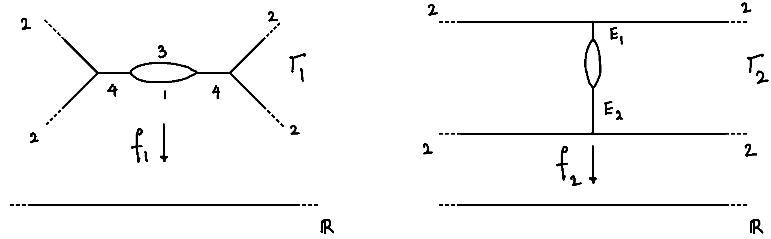
In the first case, there is an interesting constraint: the top edge of the cycle needs to have length equal to a third of the length of the borrom edge for the map to be continuous. However, in the second case, the edge lengths on the two sides of the loop are completely unconstrained by the existence of the function $f$—the existence of the function does not impose conditions on the loop. Therefore in the second case, we can move the edge lengths around to find five free parameters: four from the edge lengths and one coming from translating the piecewise linear function by a constant.

The Bieri–Groves theorem told us that, for subvarieties of $(\mathbb{C}^\star )^n$, the tropicalization detects the dimension. The set of $(C,p_1,\ldots , p_n,\varphi )$ with the data $g$ and $(a_1,\ldots , a_n)$ fixed, together forms a natural space, which is at least to first approximation, an algebraic variety. We will call it $\mathsf{M}$. Similarly, the set of tropical curves equipped with balanced, piecewise linear functions with matching data, forms a new subset which I will call $\mathsf{T}$.

Let us highlight something before carrying on. To first approximation, the space $\mathsf{M}$ can be embedded into an algebraic torus in a canonical manner and it can be tropicalized. However, the space $\mathsf{T}$ is a purely tropical object and we have made no assertion that the latter is the tropicalization of the former! The space $\mathsf{T}$ plays the role of the ambient vector space $\mathbb{R}^n$ in our first theorem, which contained the tropicalization. By using our prototype construction, with some technological upgrades, one finds that there is a continuous map

$$\begin{equation*} \mathrm{trop}:\mathsf{M}\to \mathsf{T}. \end{equation*}$$

It is not too hard to show that this map corresponds precisely to taking the data $(C_t,\varphi _t)$ and sending it the corresponding tropical pair.

If we believe that tropicalization preserves dimension, even in this more general context, then we have just argued that the codomain has larger dimension than the domain. Therefore the map cannot possibly be surjective. It follows that if one chooses the edge lengths of $E_1$ and $E_2$ generically, the data $(\Gamma _2,f_2)$ cannot come from algebraic geometry.

Harder facts

The dimension constraint above is useful for proving negatives, i.e., that there exist non-realizable tropical curves. In our argument, it’s clear where the issue comes from. A function that is linear puts a constraint on each cycle: because there are two ways to go around the cycle, if the function $\varphi$ is non-constant on the cycle, it says that the lengths of the two paths depend on each other. If the function is constant, this constraint goes away.

The following theorem says that the converse is true, and is much harder to prove.

Theorem 0.0.3.

Let $\Gamma$ be a tropical curve, and let $\varphi$ be a piecewise linear function. Assume that every vertex of $\Gamma$ has exactly three outgoing edges. If $\varphi$ is non-constant on all cycles of $\Gamma$, then $\varphi$ is realizable.

The result above was proved, in a much more general context, by Cheung, Fantini, Park, and Ulirsch 4. Ignoring the condition about the three outgoing edges at every vertex, it basically says that if the dimension argument in the previous section does not apply, then realizability holds. This is not at all obvious: why does the dimension argument see all the possible ways in which the realizability problem might fail? Nevertheless, the result is true, and the proof is a nice application of some abstract machinery: logarithmic deformation theory.

In a different direction, Speyer proved a beautiful result about the realizability of tropical curves of genus $1$ 13. If we specialize this theorem to our non-realizable example from before, one finds the following simple consequence. There are two contracted edges in the figure that are labelled as $E_1$ and $E_2$, adjacent to the cycle in the graph. As a result of Speyer’s theorem, we have the following fact:

The pair $(\Gamma _2,f_2)$ above is realizable if and only if $E_1$ and $E_2$ have the same length.

Speyer’s proof of this theorem required a sophisticated piece of algebraic geometry called non-archimedean uniformization for elliptic curves, developed by Tate. Many different proofs have been found in the 15 year since then, but the result does not appear to be elementary.

Brill–Noether theory for curves

We now discuss an application of these ideas involving tropicalization and its inversion to Brill–Noether theory, which we mentioned in passing early in this article. Let us first state the basic goal of Brill–Noether theory.

Understand the geometry of spaces parameterizing of maps from curves to projective space of a given type.

The word “understand” above includes things like knowing when such spaces are nonempty, calculating their basic invariants such as dimension or Euler characteristic, or determining topological properties such as connectedness or smoothness. The phrase “of a given type” means fixing numerical parameters. The questions in Brill–Noether theory involve three simple numerical parameters: the genus $g$ of the curve $C$, the dimension $r$ of the projective space $\mathbb{P}^r$, and the degree $d$ of the maps. The numbers combine to give the Brill–Noether number:

$$\begin{equation*} \rho (g,r,d) = g-(r+1)(g-d+r). \end{equation*}$$

If we fix a curve $C$, there is a space $W^r_d(C)$ that can be thought of as a parameter space for maps from $C$ to $\mathbb{P}^r$ of degree $d$, whose image is not contained in a hyperplane. I have suppressed a few fudge factors here, related to changes of coordinates and “base points.”

We can now state the fundamental theorem in Brill–Noether theory. Recall that the space of abstract curves $\mathcal{M}_g$ of genus $g$ has dimension $3g-3$. In what follows, we will say that a statement holds “for the general curve” if it holds for a dense subset of curves in $\mathcal{M}_g$.

The Brill–Noether theorem.

If $C$ is a general curve, the space $W^r_d(C)$ has dimension exactly $\rho (g,r,d)$.

Part of the assertion is that if $\rho (g,r,d)$ is negative, the space $W^r_d(C)$ is empty. The statement has roots in the 19th century, but was first rigorously proved in the late 20th century. As we mentioned earlier, part of this statement is accessible via an impossibility constraint—when $\rho (g,r,d)$ is negative, one has to find a graph that does not admit a certain combinatorial structure.

When $\rho (g,r,d)$ is positive, one can actually use tropical inverse problems to calculate the dimension of $W^r_d(C)$, and this was done in 9. In order to do this, one has to prove that “sufficiently many” abstract tropical curves of genus $g$ admit a map to $\mathbb{R}^r$ of genus $g$, and that the choices for maps have $\rho (g,r,d)$ dimensions worth of choices. Extracting this statement is subtle—one needs to choose the right family of graphs and check various conditions on the maps, but once the dust has settled, the task is to analyze maps

$$\begin{equation*} \Gamma \to \mathbb{R}^r \end{equation*}$$

from genus $g$ abstract tropical curves, that are built up from the balanced piecewise linear functions we saw earlier. The key question is then: do all of these maps come from algebraic geometry?

The strategy we saw in the previous discussion for curves with a piecewise linear function works perfectly well in this multivariate setting, and one can show that Cheung, Fantini, Park, and Ulirsch’s work applies perfectly, and allows us to deduce the complete Brill–Noether theorem—proving both the non-existence of maps when $\rho (g,r,d)$ is negative, but also proving the existence of maps when it is positive.

Beyond general curves

While the Brill–Noether theorem tells us precisely when maps to $\mathbb{P}^r$ do and do not exist from general curves of a given genus, it does not settle the story. For example, for every value of the genus $g$, there exist curves of genus $g$ that admit a map to $\mathbb{P}^1$ of degree $2$. Since $\rho (g,r,d)$ is negative, this is “unexpected.” In order to get a more complete picture we must go beyond the general curve, and to do this we need a way to measure the failure of a curve to be general.

One classical way to measure that failure of a curve to be general is the gonality. The gonality of a curve $C$ is the smallest degree of a map from that curve to $\mathbb{P}^1$. The gonality takes values between $2$ and $\lfloor \frac{g+3}{2}\rfloor$. The curves of gonality $2$ are called hyperelliptic and appear in numerous contexts. Classical geometry had given us an understanding of curves of gonality $2$, $3$, and $4$ in all genus, but the general case remained open.

In 2016, Pflueger revisited this problem from the point of view of tropical geometry 12. For each value $k$ of the gonality, Pflueger studied carefully-chosen tropical curves $\Gamma _g$, one in each genus. These were known to be tropicalizations of algebraic curves of gonality $k$. He then performed a beautiful combinatorial analysis to calculate the dimension of a space $W^r_d(\Gamma _g)$—a purely tropical geometric object that plays the role of $W^r_d(C)$ above. The combinatorial analysis was done via the combinatorics of chip-firing and Young tableaux.

The result of the combinatorial analysis was a formula for the dimension of $W^r_d(\Gamma _g)$, which we will call $\rho _k(g,r,d)$. The definition of this number is a little complicated but similar to the $\rho (g,r,d)$ above. Together with Jensen, we proved a $k$-gonal refinement of the classical Brill–Noether theorem 9.

The Brill–Noether theorem.

If $C$ is a general curve of gonality $k$, the space $W^r_d(C)$ has dimension exactly $\rho _k(g,r,d)$.

The proof of this theorem involved a solution to a tropical inverse problem. Points in the space $W^r_d(\Gamma _g)$ for Pflueger’s graphs $\Gamma _g$ turn out to give rise to maps

$$\begin{equation*} \Gamma _g\to \mathbb{R}^r, \end{equation*}$$

which are balanced piecewise linear functions in each coordinate—just as we saw when discussing the the tropical inverse problem. However, in each coordinate, they behave more like the badly behaved examples with contracted cycles than the nicer examples where the earlier results of Cheung, Fantini, Park, and Ulirsch apply.

By combining Speyer’s theorem on realizablity with results in logarithmic geometry and non-archimedean analysis that had been developed in the preceding years, we solved the relevant tropical inverse problem to show that Pflueger’s analysis on the tropical side correctly predicted the dimensions of the corresponding algebraic varieties.

My goal was to convey a sense of what these tropical inverse problems look like, and what kind of information their answers can reveal. However, I should say that in the years since these results were first proved, the subject of Brill–Noether theory beyond the general curve has flourished, with many new beautiful results using a variety of different and new methods. See the survey 8 and references therein.

References

- [1]
- Federico Ardila, The geometry of matroids, Notices Amer. Math. Soc. 65 (2018), no. 8, 902–908. MR3823027,
Show rawAMSref
\bib{Ard18}{article}{ author={Ardila, Federico}, title={The geometry of matroids}, journal={Notices Amer. Math. Soc.}, volume={65}, date={2018}, number={8}, pages={902--908}, issn={0002-9920}, review={\MR {3823027}}, } - [2]
- Matthew Baker, Specialization of linear systems from curves to graphs, Algebra Number Theory 2 (2008), no. 6, 613–653, DOI 10.2140/ant.2008.2.613. With an appendix by Brian Conrad. MR2448666,
\bib{Bak08}{article}{ author={Baker, Matthew}, title={Specialization of linear systems from curves to graphs}, note={With an appendix by Brian Conrad}, journal={Algebra Number Theory}, volume={2}, date={2008}, number={6}, pages={613--653}, issn={1937-0652}, review={\MR {2448666}}, doi={10.2140/ant.2008.2.613}, } - [3]
- Melody Chan, Moduli spaces of curves: classical and tropical, Notices Amer. Math. Soc. 68 (2021), no. 10, 1700–1713, DOI 10.1090/noti2360. MR4323846,
\bib{Cha21}{article}{ author={Chan, Melody}, title={Moduli spaces of curves: classical and tropical}, journal={Notices Amer. Math. Soc.}, volume={68}, date={2021}, number={10}, pages={1700--1713}, issn={0002-9920}, review={\MR {4323846}}, doi={10.1090/noti2360}, } - [4]
- Man-Wai Cheung, Lorenzo Fantini, Jennifer Park, and Martin Ulirsch, Faithful realizability of tropical curves, Int. Math. Res. Not. IMRN 15 (2016), 4706–4727, DOI 10.1093/imrn/rnv269. MR3564625,
\bib{CFPU}{article}{ author={Cheung, Man-Wai}, author={Fantini, Lorenzo}, author={Park, Jennifer}, author={Ulirsch, Martin}, title={Faithful realizability of tropical curves}, journal={Int. Math. Res. Not. IMRN}, date={2016}, number={15}, pages={4706--4727}, issn={1073-7928}, review={\MR {3564625}}, doi={10.1093/imrn/rnv269}, } - [5]
- Filip Cools, Jan Draisma, Sam Payne, and Elina Robeva, A tropical proof of the Brill-Noether theorem, Adv. Math. 230 (2012), no. 2, 759–776, DOI 10.1016/j.aim.2012.02.019. MR2914965,
\bib{CDPR}{article}{ author={Cools, Filip}, author={Draisma, Jan}, author={Payne, Sam}, author={Robeva, Elina}, title={A tropical proof of the Brill-Noether theorem}, journal={Adv. Math.}, volume={230}, date={2012}, number={2}, pages={759--776}, issn={0001-8708}, review={\MR {2914965}}, doi={10.1016/j.aim.2012.02.019}, } - [6]
- Phillip Griffiths and Joseph Harris, On the variety of special linear systems on a general algebraic curve, Duke Math. J. 47 (1980), no. 1, 233–272. MR563378,
\bib{GH80}{article}{ author={Griffiths, Phillip}, author={Harris, Joseph}, title={On the variety of special linear systems on a general algebraic curve}, date={1980}, issn={0012-7094}, journal={Duke Math. J.}, volume={47}, number={1}, pages={233\ndash 272}, url={http://projecteuclid.org/euclid.dmj/1077313873}, review={\MR {563378}}, } - [7]
- David Jensen, Chip firing and algebraic curves, Notices Amer. Math. Soc. 68 (2021), no. 11, 1875–1881, DOI 10.1090/noti2378. MR4339420,
\bib{Jen21}{article}{ author={Jensen, David}, title={Chip firing and algebraic curves}, journal={Notices Amer. Math. Soc.}, volume={68}, date={2021}, number={11}, pages={1875--1881}, issn={0002-9920}, review={\MR {4339420}}, doi={10.1090/noti2378}, } - [8]
- David Jensen and Sam Payne, Recent Developments in Brill-Noether Theory, Preprint, arXiv:2111.00351, 2021.,
\bib{JP21}{eprint}{ author={Jensen, David}, author={Payne, Sam}, title={{Recent Developments in Brill-Noether Theory}}, date={2021}, arxiv={2111.00351}, } - [9]
- David Jensen and Dhruv Ranganathan, Brill-Noether theory for curves of a fixed gonality, Forum Math. Pi 9 (2021), Paper No. e1, 33, DOI 10.1017/fmp.2020.14. MR4199236,
\bib{JR21}{article}{ author={Jensen, David}, author={Ranganathan, Dhruv}, title={Brill-Noether theory for curves of a fixed gonality}, journal={Forum Math. Pi}, volume={9}, date={2021}, pages={Paper No. e1, 33}, review={\MR {4199236}}, doi={10.1017/fmp.2020.14}, } - [10]
- Diane Maclagan and Bernd Sturmfels, Introduction to tropical geometry, Graduate Studies in Mathematics, vol. 161, American Mathematical Society, Providence, RI, 2015, DOI 10.1090/gsm/161. MR3287221,
\bib{MS15}{book}{ author={Maclagan, Diane}, author={Sturmfels, Bernd}, title={Introduction to tropical geometry}, series={Graduate Studies in Mathematics}, volume={161}, publisher={American Mathematical Society, Providence, RI}, date={2015}, pages={xii+363}, isbn={978-0-8218-5198-2}, review={\MR {3287221}}, doi={10.1090/gsm/161}, } - [11]
- Grigory Mikhalkin, Enumerative tropical algebraic geometry in , J. Amer. Math. Soc. 18 (2005), no. 2, 313–377, DOI 10.1090/S0894-0347-05-00477-7. MR2137980,
\bib{Mi05}{article}{ author={Mikhalkin, Grigory}, title={Enumerative tropical algebraic geometry in $\mathbb {R}^2$}, journal={J. Amer. Math. Soc.}, volume={18}, date={2005}, number={2}, pages={313--377}, issn={0894-0347}, review={\MR {2137980}}, doi={10.1090/S0894-0347-05-00477-7}, } - [12]
- Nathan Pflueger, Brill-Noether varieties of -gonal curves, Adv. Math. 312 (2017), 46–63, DOI 10.1016/j.aim.2017.01.027. MR3635805,
\bib{Pfl17}{article}{ author={Pflueger, Nathan}, title={Brill-Noether varieties of $k$-gonal curves}, journal={Adv. Math.}, volume={312}, date={2017}, pages={46--63}, issn={0001-8708}, review={\MR {3635805}}, doi={10.1016/j.aim.2017.01.027}, } - [13]
- David E. Speyer, Parameterizing tropical curves I: Curves of genus zero and one, Algebra Number Theory 8 (2014), no. 4, 963–998, DOI 10.2140/ant.2014.8.963. MR3248991,
\bib{Spe14}{article}{ author={Speyer, David E.}, title={Parameterizing tropical curves I: Curves of genus zero and one}, journal={Algebra Number Theory}, volume={8}, date={2014}, number={4}, pages={963--998}, issn={1937-0652}, review={\MR {3248991}}, doi={10.2140/ant.2014.8.963}, } - [14]
- R. Vakil, The moduli space of curves and Gromov-Witten theory, Enumerative invariants in algebraic geometry and string theory, 2008, pp. 143–198. MR2493586,
\bib{Vak06}{incollection}{ author={Vakil, R.}, title={The moduli space of curves and {G}romov-{W}itten theory}, date={2008}, booktitle={Enumerative invariants in algebraic geometry and string theory}, series={Lecture Notes in Math.}, volume={1947}, publisher={Springer, Berlin}, pages={143\ndash 198}, url={https://doi.org/10.1007/978-3-540-79814-9_4}, review={\MR {2493586}}, } - [15]
- Ravi Vakil, The moduli space of curves and its tautological ring, Notices Amer. Math. Soc. 50 (2003), no. 6, 647–658. MR1988577,
\bib{Vak03}{article}{
author={Vakil, Ravi},
title={The moduli space of curves and its tautological ring},
journal={Notices Amer. Math. Soc.},
volume={50},
date={2003},
number={6},
pages={647--658},
issn={0002-9920},
review={\MR {1988577}},
}
Dhruv Ranganathan is an associate professor of mathematics at the University of Cambridge. His email address is dr508@cam.ac.uk.
Article DOI: 10.1090/noti2735
Credits
The opening image is courtesy of bgblue via Getty.
Figures 1–9 are courtesy of the author.
Photo of Dhruv Ranganathan is courtesy of Rachael Boyd.