The Quintic, the Icosahedron, and Elliptic Curves

There is a remarkable relationship between the roots of a quintic polynomial, the icosahedron, and elliptic curves. This discovery is principally due to Felix Klein (1878), but Klein’s marvellous book 9 misses a trick or two, and doesn’t tell the whole story. The purpose of this article is to present this relationship in a fresh, engaging, and concise way. We will see that there is a direct correspondence between:

•

“Evenly ordered” roots $(x_1, \ldots , x_5)$ of a Brioschi quintic$$\begin{equation} X^5 + 10BX^3 + 45B^2X + B^2 = 0, {\tag{1}} \end{equation}$$

•

Points on the icosahedron, and

•

Elliptic curves equipped with a primitive basis for their 5-torsion, up to isomorphism.

Moreover, this correspondence gives us a very efficient direct method to actually calculate the roots of a general quintic! For this, we’ll need some tools both new and old, such as Cremona and Thongjunthug’s complex arithmetic geometric mean 3, and the Rogers-Ramanujan continued fraction 512. These tools are not found in Klein’s book, as they had not been invented yet!

If you are impatient, skip to the end to see the algorithm.

If not, join me on a mathematical carpet ride through the mathematics of the last four centuries. Along the way we will marvel at Kepler’s Platonic model of the solar system from 1597, witness Gauss’ excitement in his diary entry from 1799, and experience the atmosphere in Trinity College Hall during the wonderful moment Ramanujan burst onto the scene in 1913.

For the approach I present here, I have learnt the most from Klein’s book itself together with the new introduction and commentary by Slodowy 9, as well as 25811.

Arnold’s Topological Proof of the Unsolvability of the Quintic

We are all familiar with the formula for the roots $x_1, x_2$ of a quadratic polynomial $X^2 + aX + b = 0$, namely

$$\begin{equation} x = \frac{-a \pm \sqrt {a^2 - 4b}}{2}. {\tag{2}} \end{equation}$$

Perhaps we are also familiar with Cardano’s formula (1545) for the roots of a cubic polynomial $X^3 + aX + b = 0$,

$$\begin{equation} x = c - \frac{a}{3c}, \quad \quad c = \sqrt [3]{-\frac{b}{2} + \sqrt {\frac{b^2}{4} + \frac{a^3}{27}}}. {\tag{3}} \end{equation}$$

There is a similar formula for the roots of a quartic polynomial, due to Ferrari (1545). We say formulas like 2 and 3 express the roots of a polynomial in terms of radicals, since the only ingredients necessary are the usual algebraic operations ($+$, $-$, $\cdot$, $/$) and extraction of $n$th roots.

It is also commonly known that Ruffini (1799) and Abel (1824) showed that there is no such radical formula for the roots $x_i$ of a general quintic equation. The standard modern way to understand these results is the algebraic framework of Galois (1832). Namely, we associate to a specific polynomial

$$\begin{equation} P = X^n + a_1 X^{n-1} + a_2 X^{n-2} + \cdots + a_{n-1} X + a_n {\tag{4}} \end{equation}$$

a finite group $G$, the Galois group of $P$ ,which is a certain subgroup of the group $S_n$ of permutations of the roots $x_1, \ldots , x_n$ of $P$. Galois showed that there is a radical formula for $x_i(a_1, \ldots , a_n)$ if and only if $G$ is a solvable group (a tower built from iteratively stacking finite cyclic groups on top of each other, i.e., “built from epicycles” as Ptolemy might have put it). Now, the Galois group of a general quintic is $S_5$, which is not solvable. Therefore, there is no radical formula for the roots of a general quintic.

Galois’ approach is elegant but requires a semester’s worth of abstract algebra to understand. In 1963, the Russian mathematician Vladimir Arnold gave an alternative topological proof of the unsolvability of the quintic in a series of lectures to high school kids in Moscow. In Arnold’s approach, instead of focusing on finding an algebraic formula for the roots of a specific polynomial $P$ as in 4, one considers the collection of all polynomials of degree $n$ as a topological space:

$$\begin{equation*} \operatorname {Poly}_n = \{\mathrm{polynomials}\; X^n + a_1 X^{n-1}+ \cdots + a_{n-1}X + a_n,a_1, \ldots , a_n \in \mathbb{C} \}. \end{equation*}$$

To each polynomial $P \in \operatorname {Poly}_n$ we may associate the unordered set $\{x_1, \ldots , x_n\}$ of its roots, so that we have a covering space

$$\begin{align*} \operatorname {Roots}& \twoheadrightarrow \operatorname {Poly}_n \\ \{x_1, \ldots , x_n\} & \mapsto \prod _{i=1}^n (X - x_i) \end{align*}$$

which is branched over the discriminant locus $D \subset \operatorname {Poly}_n$ of polynomials with multiple roots, and is an $S_n$-principal bundle over the complement $\mathcal{P}_n = \operatorname {Poly}_n \setminus D$.

If we start at some fixed basepoint polynomial $P_0 \in \mathcal{P}_n$, and move along a path in $\mathcal{P}_n$, the roots of the polynomial move around (see Figure 1). If we loop back to $P_0$, then they will have undergone a permutation. We have established a monodromy map

$$\begin{equation} \pi _1(\mathcal{P}_n, P_0) \rightarrow S_n {\tag{5}} \end{equation}$$

which in fact classifies the covering space $\mathcal{P}_n$.

(Note how this approach is more geometric than that of Galois. Instead of caring only about the permutations of the roots, we also care about the journey they undertook to accomplish that permutation.)

Arnold’s insight was to show that if there is a radical formula for the roots of a general polynomial, then the “dance of the roots” cannot be overly complex, in the sense that the image of the monodromy map must be a solvable subgroup of $S_n$. But, for example, the 1-parameter Brioschi family of quintics

$$\begin{equation*} P_B (X) = X^5 + 10B X^3 + 45B^2X + B^2, \quad B \in \mathbb{C} \end{equation*}$$

has monodromy group $A_5$ (see Figure 1), which is certainly not solvable since it is simple, as we will see by relating it to the icosahedron in the next section. Hence the unsolvability of the quintic.

In fact, after some algebraic manipulations involving at most two square roots 2, Theorem 6.6, finding the roots of the general quintic

$$\begin{equation} X^5 + a_1 X^4 + a_2 X^3 + a_3X^2 + a_4 X + a_5=0 {\tag{6}} \end{equation}$$

reduces to finding the roots of the Brioschi quintic⁠¹ $P_B$ for a certain $B \in \mathbb{C}$.

¹

Using the Brioschi quintic as normal form is one trick which Klein missed, as he instead used a different form — the Bring-Jerrard quintic — where the maximal number of coefficients $a_i$ in 6 are zero.

✖

Figure 1.

When the Brioschi parameter loops around $B=0$ along the blue loop $\sigma$ as shown on the left, the roots undergo the cyclic permutation $(14352)$ as shown on the right. In a similar way, when $B$ loops around $B=-1/1728$ along the red loop $\gamma$, the roots undergo the cyclic permutation $(153)$. These permutations generate $A_5$.

Enter the Icosahedron

Now for a wonderful fact: we will show that there is a natural correspondence between the set of “evenly ordered” d5-tuples $(x_1, \ldots , x_5)$ of roots of a Brioschi quintic $P_B$, and the set of points on the icosahedron!

To understand this, recall that the icosahedron

$$\begin{equation*} I \subset \mathbb{R}^3, \end{equation*}$$

that most enigmatic of the Platonic solids, has 30 edges, 20 equilateral faces, and 12 vertices. If we make the identification $\mathbb{R}^3 = \mathbb{C} \times \mathbb{R}$, we can take the vertices to be situated at:

$$\begin{equation} (0, \pm 1), \quad \pm \frac{1}{\sqrt {5}}(-2\zeta ^i, 1), \quad \zeta = e^{\frac{2 \pi i}{5}}. {\tag{7}} \end{equation}$$

Consider the group $G$ of rotational symmetries of $I$. Each nonidentity $g \in G$ is a rotation about an axis through an antipodal pair of edge midpoints, face midpoints, or vertices of $I$, with order 2, 3, and 5 respectively. In fact, $G$ is naturally isomorphic to $A_5$, the group of even permutations of 5 things. What are these 5 things that are being evenly permuted when we rotate the icosahedron? They are the 5 inscribed octahedra which have their vertices on the edge midpoints of $I$! See Figure 2.

Figure 2.

One of the 5 inscribed octahedra in the icosahedron. On the right, Kepler’s view of planetary orbits as inscribed Platonic solids from Mysterium Cosmographicum (1596).

 

This natural isomorphism between $G$ and $A_5$ gives us a nice way to see that $A_5$ is simple (and hence not solvable). This is because $G$ is simple: if a normal subgroup $N$ contains a rotation about an axis through a vertex $v$, then it contains rotations about all axes passing through vertices (since it is closed under conjugation). But a rotation about an edge midpoint equals the product of the rotations about the three vertices in a triangle adjacent to it, while a rotation about a face midpoint equals the product of the rotations about the two vertices in an edge adjacent to it. So if $N$ contains a rotation about $v$, it must be all of $G$, and similarly for edge midpoints and face midpoints. So, $G$ is simple, and therefore $A_5$ is simple.

Invariant Polynomials

Let $S^2$ denote the 2-dimensional unit sphere. Since $G$ is a group of rotational symmetries, it acts on $S^2$. Our goal in this section is to understand the quotient space $S^2 / G$, which we can think of as the “moduli space” of points on the “round icosahedron” (the soccer ball version of $I$, obtained by inflating $I$ outward onto the sphere $S^2$; see Figure 3). We are going to need a toolbox of $G$-invariant functions on $S^2$.

To write down such functions, we need to keep in mind that $S^2$ has the structure of a Riemann surface, since we can identify it with the complex projective plane

$$\begin{equation*} \mathbb{CP}^1 = \{ \text{1-dimensional linear subspaces of $\mathbb{C}^2$} \} \end{equation*}$$

via stereographic projection from the north pole,

$$\begin{align*} S^2 & \xrightarrow {\cong } \mathbb{C} \cup \{\infty \} \\ (a,b,c) & \mapsto \frac{a+bi}{1-c}, \end{align*}$$

followed by the identification

$$\begin{align*} \mathbb{C} \cup \{\infty \} & \xrightarrow {\cong } \mathbb{CP}^1 \\ z & \mapsto \mathbb{C}(z, 1) \\ \infty & \mapsto \mathbb{C}(1, 0). \end{align*}$$

In what follows, I will freely use these identifications; my preference is to use the $S^2$ picture because I want the visual image of the icosahedron in $\mathbb{R}^3$ to be front and center.

Under this identification, the $\mathrm{SO}(3)$ rotation action on $S^2$ translates into an $\mathrm{SO}(3)$ action on $\mathbb{CP}^1$, which can be explained as arising from the natural action of its double cover $\mathrm{SU}(2)$ on $\mathbb{C}^2$. We define the binary icosahedral group $\hat{G} \subset \mathrm{SU}(2)$ as the double cover of the icosahedral group $G \subset \mathrm{SO}(3)$. So, we seek $\hat{G}$-invariant homogenous polynomials on $\mathbb{C}^2$.

We have the vertex polynomial $V$ (of degree 12, vanishing on the 1-dimensional subspaces corresponding to icosahedron vertices), the face polynomial $F$ (of degree 20, vanishing on the 1-dimensional subspaces corresponding to icosahedron face midpoints), and the edge polynomial $E$ (of degree 30, vanishing on the 1-dimensional subspaces corresponding to icosahedron edge midpoints):

$$\begin{align} V &= uv(u^{10} + 11 u^5 v^5 - v^{10}) {\tag{8}}\\ F &= -u^{20} + 228(u^{15}v^5-u^5v^{15}) - 494u^{10}v^{10} - v^{20} {\tag{9}}\\ E &= u^{30} + 522(u^{25}v^5 - u^5v^{25}) - 1005(u^{20}v^{10} - u^{10}v^{20}) + v^{30} {\tag{10}} \end{align}$$

To see that these polynomials are indeed $\hat{G}$-invariant (instead of picking up phase factors when acting with $g \in \hat{G}$), it helps to realize that $G$ is generated by $R_z$ and $R_y$, the rotations about the $z-$ and $y-$axis by angles $2 \pi / 5$ and $\pi$ respectively. We can take their preimages in $\mathrm{SU}(2)$ to be

$$\begin{equation*} \hat{R}_z = \begin{pmatrix} e^{\frac{\pi i}{5}} & 0 \\ 0 & e^{-\frac{\pi i}{5}} \end{pmatrix}, \quad \hat{R}_y = \begin{pmatrix} 0 & -1 \\ 1 & 0 \end{pmatrix} \end{equation*}$$

which similarly generate $\hat{G}$, and which act on homogenous polynomials in $u, v$ as:

$$\begin{equation} \hat{R}_z\colon u \mapsto e^{-\frac{\pi i}{5}}u, v \mapsto e^{\frac{\pi i}{5}} v, \quad \hat{R}_y \colon u \mapsto v, v \mapsto -u {\tag{11}} \end{equation}$$

It is clear that our polynomials 8–10 are invariant under these transformations, so they are indeed $\hat{G}$-invariant. In fact, they generate the algebra of $\hat{G}$-invariant homogenous polynomials on $\mathbb{C}^2$.

Figure 3.

The round icosahedron and its stereographic projection. The edge midpoint $\alpha$ and face midpoint $\beta$, together with their stereographic projections $a$ and $b$, have been marked for later use.

We can play the same game with our 5 inscribed octahedra. Let $O_i$ be the vertex polynomial of the $i$th inscribed octahedron. It has degree 5 and vanishes at the 1-dimensional subspaces of $\mathbb{C}^2$ corresponding to the 8 vertices of $O_i$. We compute

$$\begin{equation*} O_1 = (u^2 + v^2)(u^2 - 2nuv - v^2)(u^2 - 2muv - v^2) \end{equation*}$$

where $m = \zeta + \zeta ^4=\frac{1}{\phi }$ and $n = \zeta ^2 + \zeta ^3 = -\phi$, with the other $O_i, i=2\ldots 5$ obtained by simply rotating $O_1$ around the $z$-axis using the $\hat{R}$-action in 11.

The Icosahedron and the Quintic

When we rotate the icosahedron, the 5 inscribed octahedra and hence their vertex polynomials $O_i$ undergo an (even) permutation. Consider the quintic

$$\begin{equation*} \prod _{i=1}^5 (X - O_i) \end{equation*}$$

whose coefficients are symmetric polynomials in the octahedral polynomials $O_i$ and hence $\hat{G}$-invariant polynomials on $\mathbb{C}^2$. If we multiply it out, we obtain a Brioschi-type quintic

$$\begin{equation*} X^5 - 10V X^3 + 45 V^2 X - E \end{equation*}$$

as the reader will verify! (The coefficients of $X^4$ and $X^2$ are invariant polynomials of degree $6$ and $18$ respectively and hence must vanish, while the coefficients of $X^3$, $X$ and $1$ are of degree 12, 24, and 30 and hence must be multiples of $V$, $V^2$, and $E$ respectively.)

Let us make this correspondence between points on the icosahedron and ordered roots of a Brioschi quintic clear and precise. Consider the rationalized octahedral functions

$$\begin{equation*} x_i = - \frac{V^2}{E} O_i, \quad i = 1\ldots 5. \end{equation*}$$

They are of degree zero in $u$ and $v$. Therefore, away from the edge midpoints, they are well-defined complex-valued functions on $S^2$. In other words, to each point $z$ on the “round icosahedron” $S^2$ (excluding edge midpoints), we can associate an ordered tuple $(x_1(z), \ldots , x_5(z))$ of 5 complex numbers! We map these 5 numbers to the quintic

$$\begin{equation} P_{\{x_i\}} = \prod _{i=1}^5 (X - x_i(z)) {\tag{12}} \end{equation}$$

thereby forgetting their ordering. If we multiply out this quintic, we find that it is a Brioschi quintic

$$\begin{equation*} P_B = X^5 + 10BX^3 + 45B^2 X + B^2 \end{equation*}$$

with Brioschi parameter $B(z) = -V^5/E^2$! See Figure 4. In summary, we have:

Theorem 1.

The map

$$\begin{equation*} z \mapsto (x_1 (z), \ldots , x_5(z)) \end{equation*}$$

is an $A_5$-equivariant bijection between points on the round icosahedron (minus edge midpoints) and evenly ordered (defined below) roots of Brioschi quintics $P_B$ with Brioschi parameter $B(z) = -V^5 / E^2$. In other words, it is an explicit equivariant isomorphism of covering spaces:

$$\begin{equation*} \vcenter{\img[][195pt][76pt][{\renewcommand{\arraystretch}{1} \setlength{\unitlength}{1.0pt} \setlength{\extrarowheight}{0.0pt}\begin{tikzpicture}[xscale=4, yscale=2] \node(A) at (0,0) {$S^2 \setminus\{\text{edge midpoints}\}$}; \node(B) at (1,0) {$\operatorname{EvOrRoots}$}; \node(C) at (0,-1) {$S^2 \setminus\{\infty\}$}; \node(D) at (1,-1) {$\text{Brioschi quintics}$}; \draw[->] (A) -- node[above]{$\cong$} (B); \draw[->>] (A) -- node[left]{$B$} (C); \draw[->] (C) -- node[below]{$\cong$} (D); \draw[->>] (B) -- node[right]{$P$} (D); \end{tikzpicture}}]{Images/img3fb2962dee59206fac13d29d499ebf72.svg}} \end{equation*}$$

Figure 4.

The Brioschi parameter $B(z)$ on $S^2$. The absolute value maps to the brightness, while the argument maps to the hue. Note the zeros of $B$ at the vertices of the icosahedron, and the poles at the edge midpoints.

The only subtlety here is the notion of an “evenly” ordered set of roots of a Brioschi quintic $P_B$. We need this because there are 60 points on a generic orbit $A_5 \cdot z$ in the icosahedron, while there are 120 ways to order the 5 roots $x_1, \ldots , x_5$ of the quintic $P_B$. We call an ordering of the roots of a generic Brioschi quintic $P_B$ even if, as $B$ approaches $0$ through positive real values (which implies that $z$ approaches a vertex of the icosahedron) and track the roots continuously, the roots end up in an even permutation of the numbering shown in Figure 1.

Theorem 1 tells us that in order to find the roots of a Brioschi quintic $P_B$ for some Brioschi parameter $B \in \mathbb{C}$, we need to find a point $z$ on the icosahedron such that $-V^5(z) / E^2(z) = B$. Then our 5 ordered roots will be given by the 5 octahedral numbers $x_i(z)$. Actually calculating $z$ in terms of $B$ is hard (we need to solve a polynomial equation of degree 60), but it can be done efficiently using elliptic curves, as we will see shortly!

A Polynomial Relation

But first, let’s return to the subject of invariant polynomials on the icosahedron for a moment, as there is an important relation between $V$, $E$, and $F$ which we will need later. The point is that these are polynomials on $\mathbb{C}^2$, and three polynomials on a 2-dimensional space must satisfy a relation. The first opportunity for this relation to occur is in degree 60, and indeed we have:

$$\begin{equation} E^2 + F^3 = 1728 V^5 {\tag{13}} \end{equation}$$

This reminds us of modular forms, where the Eisenstein series satisfies

$$\begin{equation*} E_6^2 - E_4^3 = 1728 \Delta . \end{equation*}$$

This is the first clue that the icosahedron has something to do with moduli spaces of elliptic curves. But for now, what we need to get out of 13 is that it tells us that

$$\begin{equation*} B(z) = - \frac{V^5}{E^2} = -\frac{V^5}{1728 V^5 - F^3} \end{equation*}$$

so that $B$ sends vertices to $0$, edge midpoints to $\infty$, and face midpoints to $-1/1728$. This uniquely characterizes it as a holomorphic map from $S^2$ to $S^2$.

Enter Elliptic Curves

Expressing a number “in terms of radicals” implies having access to the roots of unity, i.e., the $n$-torsion points (points $p$ such that $np = 0$) in the nonzero complex numbers $\mathbb{C}^*$, thought of as an additive abelian group. In the nineteenth century, mathematicians discovered that the set of points on an elliptic curve, i.e., the set $E$ of complex solutions to a cubic equation of the form

$$\begin{equation} y^2 = 4x^3 - g_2 x - g_3 {\tag{14}} \end{equation}$$

also forms an abelian group (once one works projectively). It was natural to speculate that, while the roots of a quintic could not be expressed in terms of $n$-torsion points on the circle, perhaps they could be expressed in terms of the $5$-torsion points of an elliptic curve somehow associated with the quintic. Remarkably, this is precisely what Hermite (1858) and Kiepert (1878) managed to do! To quote McKean and Moll 10:

In this way, the solution of the general equation of degree 5 is made to depend upon the equations for the division of periods of the elliptic functions, as they used to say.

Hermite and Kiepert worked with the Bring-Jerrard form of the quintic, and their final expression for the roots of the quintic in terms of the 5-torsion points of an elliptic curve is, to this humble author, a bit convoluted and indirect. I will present my own streamlined and modernized form of Klein’s approach (1878) 9. We will see that the 60 evenly ordered 5-tuples of roots $(x_1, \ldots , x_5)$ of a Brioschi quintic directly correspond to the 60 equivalence classes of primitive bases (not points themselves) for the 5-torsion points of an elliptic curve!

Moduli Spaces of Elliptic Curves

In the previous section we found that the icosahedron is a 60-sheeted $A_5$ equivariant covering space of $S^2$ via the Brioschi map $B$. And moreover, we found that away from the edge midpoints, this covering space is explicitly isomorphic to the covering space of evenly ordered roots of Brioschi quintics.

Besides the icosahedron, there is another 60-sheeted $A_5$-equivariant covering space of $S^2$ occurring in nature: the moduli space $X(5)$ of elliptic curves equipped with a primitive basis for their 5-torsion!

Recall that an elliptic curve $E \subset \mathbb{CP}^2$ given by a cubic equation as in 14 identifies holomorphically with $\mathbb{C}/\Lambda$, the quotient of $\mathbb{C}$ by some rank 2 lattice $\Lambda \subset \mathbb{C}$. So, topologically, $E$ looks like a doughnut. Moreover, under this identification the addition operation on $E$ is just the standard addition in $\mathbb{C} / \Lambda$. Therefore,

$$\begin{equation*} \text{5-torsion points of $E$} \cong \mathbb{Z}/5\mathbb{Z} \times \mathbb{Z} / 5 \mathbb{Z}. \end{equation*}$$

Let $p,q$ be 5-torsion points in $\mathbb{C} / \Lambda$ and let $\omega _1, \omega _2 \in \mathbb{C}, \operatorname {Im}(w_1/w_2) > 0$ be generators of $\Lambda$. Since the equivalence classes $[\omega _1/5], [\omega _2/5]$ generate the 5-torsion of $\mathbb{C} / \Lambda$, we can write

$$\begin{align*} p &= a_1 [\omega _1/5] + a_2 [\omega _2/5] \\ q &= b_1 [\omega _1/5] + b_2 [\omega _2/5] \end{align*}$$

for some matrix

$$\begin{equation*} \gamma \in \begin{pmatrix} a_1 & a_2 \\ b_1 & b_2 \end{pmatrix} \in \mathrm{GL}_2(\mathbb{Z}, \mathbb{Z}/5\mathbb{Z}). \end{equation*}$$

We say that $(p,q)$ is a primitive basis for the 5-torsion of $E$ if $\det \gamma \equiv 1 \mod 5$. Write

$$\begin{equation*} X(5) = \{ (E, (p, q)) \} / \sim \end{equation*}$$

for the set of equivalence classes (“moduli space”) of pairs $(E, (p,q))$ where $E$ is a complex elliptic curve and $(p,q)$ is a primitive basis for its 5-torsion (see 4). Two such pairs $(E, (p,q))$ and $(E', (p',q'))$ are equivalent if there is an isomorphism $E \rightarrow E'$ which carries $(p,q) \mapsto (p', q')$.

Write $X(1)$ for the “vanilla” moduli space of elliptic curves (no extra torsion information tagged on), and $\mathbb{H} = \{ \tau \in \mathbb{C} : \operatorname {Im}(\tau ) > 0 \}$ for the upper half plane. Thinking of an elliptic curve as a quotient $\mathbb{C} / \mathbb{Z} \oplus \mathbb{Z} \tau$ for some $\tau \in \mathbb{H}$, we can identify these moduli spaces as:

$$\begin{equation*} X(1) \cong \mathbb{H}^* \big / SL(2, \mathbb{Z}), \quad X(5) \cong \mathbb{H}^* \big / \Gamma (5). \end{equation*}$$

Here, $\mathbb{H}^* = \mathbb{H} \cup \mathbb{Q} \cup \{i \infty \}$ is the extended upper half plane (the extra “cusp” points $\mathbb{Q} \cup \{i \infty \}$ are needed to get a compact moduli space; they contribute a single point to the quotient in $X(1)$ and 12 points in $X(5)$) and

$$\begin{equation*} \Gamma (5) = \left\{\,\begin{pmatrix} a & b \\ c & d \end{pmatrix} \in \mathrm{SL}(2, \mathbb{Z}) : \begin{pmatrix} a & b \\ c & d \end{pmatrix} \equiv \begin{pmatrix} 1 & 0 \\ 0 & 1 \end{pmatrix} , \operatorname {mod} 5 \,\right\} \end{equation*}$$

is the principal congruence subgroup of level 5. (The congruence relation is done independently entrywise, so the requirement is that $a \equiv 1 \pmod {5}$, $b \equiv 0 \pmod {5}$, $c\equiv 0 \pmod {5}$ and $d \equiv 1 \pmod {5})$.

Permutation Wizardry

Now, $\Gamma (5)$ is a normal subgroup of $\Gamma \coloneq \mathrm{SL}(2, \mathbb{Z})$, and so we can form the quotient group

$$\begin{equation*} \Gamma / \Gamma (5) \cong \mathrm{PSL}(2, \mathbb{Z} / 5\mathbb{Z}). \end{equation*}$$

The magic is that $\mathrm{PSL}(2, \mathbb{Z} / 5\mathbb{Z})$ is isomorphic to $A_5$! We will need to understand this isomorphism explicitly in terms of the action of $A_5$ on the five inscribed octahedra⁠².

²

I learned this argument from David Speyer and Beren Gunsolus 13.

✖

The vertices of an inscribed octahedron $O_i$ are located at edge midpoints of the icosahedron $I$. Therefore, $O_i$ partitions the vertices of $I$ into pairs, and hence encodes a fixed-point free involution of the 12 vertices of $I$. This involution commutes with the map $p \rightarrow -p$, and so we conclude that each inscribed octahedron $O_i$ encodes (and is in fact encoded by) a fixed-point free involution $o_i$ of the 6 vertex axes of $I$.

On the other hand, $PSL(2, \mathbb{Z}/5 \mathbb{Z})$ acts naturally on projective space

$$\begin{equation*} \mathbb{P}^1(\mathbb{Z}/5\mathbb{Z}) = \{ 0, 1, 2, 3, 4, \infty \}, \end{equation*}$$

which also consists of 6 things. So, let us identify the six vertex axes of the icosahedron in $\mathbb{R}^3$ with $\mathbb{P}^1(\mathbb{Z}/5\mathbb{Z})$ in the natural way:

$$\begin{align*} \mathbb{R} (-2 \zeta ^k, 1) & \mapsto k, \quad k=0\ldots 4 \\ \mathbb{R} (0, 0, 1) &\mapsto \infty . \end{align*}$$

In this way $PSL(2, \mathbb{Z}/5\mathbb{Z}) \subset S_6$ acts by conjugation on the 5 octahedral involutions $o_i \in S_6$, and it turns out that it permutes them evenly, giving our isomorphism $PSL(2, \mathbb{Z}/5\mathbb{Z}) \cong A_5$.

Let us pre- and post-compose this isomorphism with the natural isomorphisms $\Gamma / \Gamma (5) \cong \mathrm{PSL}(2, \mathbb{Z} / 5\mathbb{Z})$ and $A_5 \cong G$ and record the result explicitly for later use.

Lemma 1.

The explicit isomorphism

$$\begin{align*} \Gamma / \Gamma (5) & \rightarrow G, \end{align*}$$

at the level of generators, sends

$$\begin{align*} T &\mapsto R_z \\ S &\mapsto R_\alpha , \end{align*}$$

where $T(\tau ) = \tau +1$ and $S(\tau )=-\frac{1}{\tau }$, and $R_z (z) =\zeta z$ and $R_\alpha (z) = \frac{nz + 1}{z-n}$ are rotations by $\frac{2\pi }{5}$ and $\pi$ counterclockwise about the positive z-axis and the axis through the edge midpoint $\alpha$ shown in Figure 3 respectively.

An Isomorphism of Covering Spaces

The isomorphism $PSL(2, \mathbb{Z}/5\mathbb{Z}) \cong A_5$ means that the forgetful map

$$\begin{equation*} \pi : X(5) \twoheadrightarrow X(1) \end{equation*}$$

is an $A_5$-equivariant 60-sheeted covering space of $X(1)$. Note that we can also make our own direct count of the sheets in the covering. Given an elliptic curve $E \in X(1)$, there are $480 = 24 \times 20$ pairs $(p,q)$ which form a basis for the 5-torsion, since the only constraint is that $p \neq 0$ and $q \notin \{0, p, 2p, 3p, 4p\}$. Of these 480 pairs, exactly 120 will be a primitive basis. If $E$ is a generic elliptic curve, then we must also account for its solitary nontrivial automorphism $p \mapsto -p$. So there are 60 points in a generic fiber.

Now, the moduli space $X(1)$ of elliptic curves identifies with $S^2$,

$$\begin{equation*} j \colon \mathbb{H}^* \big / SL(2, \mathbb{Z}) \xrightarrow {\cong } S^2, \end{equation*}$$

via the $j$-invariant of an elliptic curve:

$$\begin{align*} j(\tau ) &= \frac{1728 g_2^3}{g_2^3 - 27 g_3^2} \\ &= \frac{1}{q} + 744 + 196884 q^2 + \cdots . \end{align*}$$

Here, $q = e^{2 \pi i \tau }$ and $g_2$ and $g_3$ are the coefficients appearing in the equation 14 for an elliptic curve $E$. If we identify $E$ with the quotient of $\mathbb{C}$ by a lattice $\Lambda _\tau = \mathbb{Z} \oplus \mathbb{Z}\tau$, where $\tau \in \mathbb{H}$, then they are computed in terms of $\tau$ as

$$\begin{equation*} g_2 = 60 \sideset{}{'}{\sum }_{\omega \in \Lambda _\tau } \frac{1}{\omega ^4}, \quad g_3 = 140 \sideset{}{'}{\sum }_{\omega \in \Lambda _\tau } \frac{1}{\omega ^6}, \end{equation*}$$

where the primes on the sums means leaving out $\omega = 0$ from the sum.

Ok, so now we know that $X(5)$ is an $A_5$-equivariant covering space of $S^2$. If $E_j$ is an elliptic curve with invariant $j \in S^2$, then the number of points in the fiber is given by

$$\begin{equation*} | \pi ^{-1} (j) | = \frac{120}{|\operatorname {Aut}(E_j)|}, \end{equation*}$$

as we explained above. A generic elliptic curve has automorphism group $\mathbb{Z} / 2 \mathbb{Z}$, corresponding to the involution $p \mapsto -p$, but precisely two curves have more symmetry, namely those constructed from the square lattice ($j = 1728$) and the hexagonal lattice ($j = 0$):

$$\begin{align*} \operatorname {Aut}(\mathbb{C}\big /\mathbb{Z} \oplus \mathbb{Z}i) &\cong (\mathbb{Z} / 2 \mathbb{Z})^2 \\ \operatorname {Aut}(\mathbb{C}\big /\mathbb{Z} \oplus \mathbb{Z}e^{\pi i / 3}) &\cong \mathbb{Z} / 2 \mathbb{Z} \times \mathbb{Z} / 3 \mathbb{Z}. \end{align*}$$

We should also figure out how many cusp points there are (i.e., count points in the fiber over $j=\infty$). This requires counting the number of orbits of the action of $\mathrm{SL}(2, \mathbb{Z})$ on the extended rationals $\mathbb{Q} \cup \{i \infty \}$. A quick calculation shows there are 12 of these, whose representatives we can take to be:

$$\begin{equation} \mathrm{cusps} = \left\{\,i\infty , \frac{2}{5}\right\} \cup \left\{\frac{k}{2} : k=0 \ldots 9 \right\} {\tag{15}} \end{equation}$$

So, in summary, $X(5)$ is an $A_5$-equivariant branched covering space of $S^2$, with three branch points $j=1728$, $j=0$ and $j=\infty$ having 30, 20, and 12 elements in their fibers respectively. This implies that it is isomorphic, as a branched covering space, to the “round icosahedron” $S^2$! In particular, it has genus zero.

Tidying things up

Let’s tidy up this isomorphism of covering spaces over $S^2$ by ensuring that the branch points correspond correctly.

Instead of using $B = -V^5/E^2$ to identify the icosahedron quotient $S^2 / A_5$ with $S^2$ (which was convenient from the viewpoint of identifying points on the icosahedron with ordered roots of Brioschi quintics, but not with elliptic curves), we should use Klein’s function

$$\begin{equation} J(z) = \frac{F^3}{V^5} = \frac{1728 V^5 - E^2}{V^5} = 1728 + \frac{1}{B} {\tag{16}} \end{equation}$$

instead. (Recall the fundamental relation 13). This $J$-invariant aligns correctly with the projection $\pi : X(5) \twoheadrightarrow X(1)$, since it sends the 30 edge midpoints to $J=1728$, the 20 face midpoints to $J=0$, and the 12 vertices to $J=\infty$. Let us record this in a theorem.

Theorem 2.

There is an $A_5$-equivariant isomorphism $j_5$ of covering spaces between the moduli space $X(5)$ of elliptic curves equipped with a choice of primitive basis for their 5-torsion, and the icosahedron, such that the following diagram commutes:

$$\begin{equation} \begin{aligned} \vcenter{\img[][139pt][81pt][{\renewcommand{\arraystretch}{1} \setlength{\unitlength}{1.0pt} \setlength{\extrarowheight}{0.0pt}\begin{tikzpicture}[xscale=4, yscale=2] \node(A) at (0,0) {$\mathbb{H}^* {\big/} \Gamma(5)$}; \node(B) at (1,0) {$S^2$}; \node(C) at (0,-1) {$S^2$}; \node(D) at (1,-1) {$S^2$}; \draw[->] (A) -- node[above]{$j_5$} node[below] {$\cong$} (B); \draw[->>] (A) -- node[left]{$j$} (C); \draw[->] (C) -- node[below]{$\operatorname{id}$} (D); \draw[->>] (B) -- node[right]{$J$} (D); \end{tikzpicture}}]{Images/imgaf750b143ae0a9a2e4409b8300b4658a.svg}} \end{aligned} {\tag{17}} \end{equation}$$

Figure 5.

The map $j_5$ is an $A_5$-equivariant map from $\mathbb{H}^*/\Gamma$ to $S^2$. The standard tesselation of $\mathbb{H}^*$ by fundamental domains for $\Gamma$ is shown, together with their image on $S^2$. Images taken from 6.

$\xrightarrow {j_5}$

Let us nail down the definition of $j_5$. To make 17 commute, we know it must send:

$$\begin{align*} i\infty & \mapsto \text{a vertex} \\ i \mapsto & \mapsto \text{an edge midpoint} \\ e^\frac{2 \pi i}{3} & \mapsto \text{a face midpoint}. \end{align*}$$

Since $j_5$ is $A_5$-equivariant, it must send fixed points of the action of $A_5$ on $\mathbb{H}^*$ to fixed points of the action of $A_5$ on $S^2$. This determines $j_5$ up to some sign choices, which we now fix.

Refer to Figure 3. A rotation about the $z$-axis in $S^2$ by $\pi /5$ corresponds, by Lemma 1, to the transformation $\tau \mapsto \tau + 1$ of $\mathbb{H}^*$, whose only fixed point is $i\infty \in \mathbb{H}^*$. So, we must have $j_5(i\infty ) \in \{0, \infty \} \subset S^2$, and we make the natural choice $j_5(i\infty ) = 0$, to line up on-the-nose with $j$.

Similarly, a rotation about the $\alpha$-axis in $S^2$ by $\pi$ corresponds to the transformation $\tau \mapsto -1/\tau$ on $\mathbb{H}^*$, whose only fixed point is $\tau = i$. So, $j_5(i)$ must equal $\pm a$, and we choose the plus sign. In the same way, since rotation around $b$ by $2 \pi / 3$ equals the product $R_a R_z$ and hence corresponds to the transformation $\tau \mapsto -\frac{1}{\tau + 1}$, whose only fixed point is $\tau = e^{2 \pi i/3}$, we must have $j_5(e^\frac{2 \pi i}{3}) = \pm b$, and again we choose the plus sign.

In summary, after doing a quick calculation of the stereographic projections $\alpha$ and $\beta$ of $a$ and $b$, we are defining $j_5$ as the unique $A_5$ equivariant map $\mathbb{H}^* / \Gamma (5) \rightarrow S^2$ satisfying:

$$\begin{align} j_5(i\infty ) &= \infty \tag{18}\\ j_5 (i) &= \alpha = \sqrt {\frac{5 + \sqrt {5}}{2}} - \frac{\sqrt {5}+ 1}{2} {\tag{19}}\\ j_5(e^\frac{\pi i }{3}) &= \beta = e^{\frac{-2 \pi i}{ 10}} \frac{\sqrt {30 + 6 \sqrt {5}} - 3 - \sqrt {5}}{4}. {\tag{20}} \end{align}$$

See Figure 5. This definition is great…but it would be nice to have an explicit formula for $j_5(\tau )$, for an arbitrary point $\tau \in \mathbb{H}^*$!

Enter Ramanujan

On Sunday evening of February 2, 1913, Bertrand Russell wrote to his lover Lady Ottoline Morrell from his rooms in Trinity College Cambridge:

In Hall I found Hardy, and Littlewood in a state of wild excitement, because they believe they have discovered a second Newton, a Hindu clerk in Madras on £20 a year. He wrote to Hardy telling him of some results he has got, which Hardy thinks quite wonderful, especially as the man has had only an ordinary school education. Hardy has written to the Indian Office and hopes to get the man here at once.

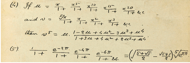
Behold the stir which Srinivasa Ramanujan (1887–1920) created when he sent his famous letter to Hardy, England’s foremost mathematician at the time, from the Port Trust Office in Madras on January 16, 1913. Figure 6 shows an extract from page 9 of his letter. In formula (4), we see that Ramanujan introduces a continued fraction

$$\begin{equation} r(q) = \dfrac{q^{\dfrac{1}{5}}}{1 + \dfrac{q}{1+ \dfrac{q^2}{1 + \dfrac{q^3}{1 + \cdots }}}} {\tag{21}} \end{equation}$$

and states an identity involving it, while in (5) we find the remarkable evaluation

$$\begin{equation} r(e^{- 2 \pi }) = \sqrt {\frac{5 + \sqrt {5}}{2}} - \frac{\sqrt {5} + 1}{2}. {\tag{22}} \end{equation}$$

Figure 6.

Extract from page 9 of Ramanujan’s first letter to Hardy on January 16, 1913.

Hardy famously wrote 7 that formulas (4) and (5) as well as a similar evaluation of $r(e^{-2 \pi \sqrt {5}})$ (from Ramanujan’s second letter to Hardy)

…defeated me completely; I had never seen anything in the least like them before. A single look at them is enough to show that they could only be written down by a mathematician of the highest class. They must be true because, if they were not true, no one would have had the imagination to invent them.

The continued fraction $r(q)$ in 21 is called the Rogers-Ramanujan continued fraction, since it had been first written down 20 years earlier by Rogers (1894), who proved some important identities regarding it. Thus Ramanujan had independently rediscovered it, and had proved some remarkable new identities of his own, such as those above.

Ramanujan and the Icosahedron

Staring at equations 19 and 22, we immediately conjecture the following relationship between the Rogers-Ramanujan continued fraction $r$ and the $j_5$ covering map from the world of elliptic curves:

$$\begin{equation} j_5 (\tau ) = r(q), \quad q = e^{2 \pi i \tau }. {\tag{23}} \end{equation}$$

This is indeed the case! From Theorem 2 and the discussion below it, all we need to do is establish equivariance of $r(q)$, thought of as a function of $\tau$!

Theorem 3 (5).

The Rogers-Ramanujan continued fraction $r$ is an $A_5$-equivariant map

$$\begin{equation*} \mathbb{H}^* / \Gamma (5) \rightarrow S^2. \end{equation*}$$

That is,

$$\begin{align} r(\tau + 1) &= R_z r(\tau ) = \zeta r(\tau ) {\tag{24}}\\ r\left(-\frac{1}{\tau }\right) &= R_\alpha r(\tau ) = \frac{1-\phi r(\tau )}{\phi + r(\tau )}, {\tag{25}} \end{align}$$

where $\phi = \frac{1 + \sqrt {5}}{2}$.

The idea of the proof is as follows. Equivariance 24 with respect to rotations about the $z$-axis follows immediately from the $q^\frac{1}{5}$ factor in the definition 21 for $r$. The transformation formula 25 for $r(-\frac{1}{\tau })$ follows from the Rogers-Ramanujan identities which allow us to write $r$ as a ratio of two theta functions, each of whose transformation properties under $\tau \mapsto -\frac{1}{\tau }$ is known.

Once we know $r$ is an $A_5$-equivariant map (and hence $r = j_5$), we immediately have Ramanujan’s beautiful formulas 22 and 20⁠³!

³

This formula appears in Ramanujan’s “lost notebook.”

✖

Indeed, the equivariance allows us to calculate $r(\tau )$ at any point $\tau \in \Gamma \cdot \{i, \rho , \infty \}$, since these map to the 62 special points on the icosahedron (12 vertices + 20 face midpoints + 30 edge midpoints). This gives us a bunch of intriguing identities! For instance, what is $r(0)$? Well,

$$\begin{align*} r(0) &= r(S(i \infty )) \\ &= R_\alpha r(i \infty ) \\ &= -\frac{1}{n} = \frac{1+\sqrt {5}}{2}. \end{align*}$$

In other words, we have

$$\begin{equation*} \frac{1}{1+\dfrac{1}{1+\dfrac{1}{1 + \cdots }}} = \frac{1+\sqrt {5}}{2}, \end{equation*}$$

which is indeed a well-known identity!

Similarly, for which $\tau$ is $r(\tau )$ equal to the edge midpoint $i \in S^2$? Well, we know that $r(i \in \mathbb{H}) = \alpha$, and we know that $R_z^2 R_\alpha R_z^2 R_\alpha R_z \cdot \alpha = i \in S^2$, therefore

$$\begin{equation*} r(T^2ST^2ST \cdot i) = i, \quad \text{i.e., } r\left(\frac{7+i}{5}\right) =i, \end{equation*}$$

and hence $r\left(\Gamma (5) \cdot \frac{7+i}{5}\right) = i$.

Gauss and the Arithmetic-Geometric Mean

We’re going to need one final ingredient before we can tie everything together. In our algorithm for finding the roots of a quintic, we will start with a quintic, do some magic, and associate to it an elliptic curve $E$ in Weierstrass form:

$$\begin{equation} E: y^2 = 4x^3 - g_2 x - g_3 {\tag{26}} \end{equation}$$

The next thing we will need is to find $\tau \in \mathbb{H}$ such that $E \cong \mathbb{C}/\mathbb{Z} \oplus \mathbb{Z} \tau$. This means we need to find a basis $\omega _1$, $\omega _2$ for the period lattice 10 $\Lambda \subset \mathbb{C}$ of $E$,

$$\begin{equation*} \Lambda = \left\{\, \int _\gamma \frac{dx}{y} : \gamma \in H_1(E, \mathbb{Z}) \,\right\}, \end{equation*}$$

and then set $\tau = \frac{\omega _2}{\omega _1}$. But we don’t want to have to calculate integrals in order to solve the quintic! How can we calculate periods efficiently?

This is where the final piece of magic enters the story. In the late 1790s, Gauss was trying to compute precisely such a period integral, namely

$$\begin{equation*} \omega = \int _{-1}^1 \frac{dx}{\sqrt {1-x^4}}. \end{equation*}$$

He was excited to discover that such period integrals can be calculated very efficently using an algorithm called the arithmetic-geometric mean (see Figure 7). Given two positive real numbers $a$ and $b$, define sequences $a_n$ and $b_n$ by starting with $a_0 = a$ and $b_0 = b$ and then setting

$$\begin{align} a_{n+1} &= \frac{1}{2}(a_n + b_n) {\tag{27}}\\ b_{n+1} &= \sqrt {a_n b_n} {\tag{28}} \end{align}$$

so that $a_{n+1}$ is the arithmetic mean of $a_n$ and $b_n$, and $b_{n+1}$ is their geometric mean. These sequences converge very rapidly (the accuracy doubles with each iteration), and the arithmetic-geometric mean of $a$ and $b$ is defined as the common limit

$$\begin{equation*} M(a,b) = \lim _{n\rightarrow \infty } a_n = \lim _{n\rightarrow \infty } b_n. \end{equation*}$$

Figure 7.

The entry in Gauss’ mathematical diary on May 30, 1799, recording his excitement at the discovery that $\omega = \pi /M(1, \sqrt {2})$. Translation from Latin: We have confirmed up to the eleventh figure that the arithmetic-geometric mean of $1$ and $\sqrt {2}$ equals $\frac{\pi }{\omega }$. Therefore, once demonstrated, a completely new field in analysis will certainly be opened.

More generally, given an elliptic curve $E$ in Weierstrass form 26 which factorizes as

$$\begin{equation*} 4x^2 - g_2 x - g_3 = 4(x-e_1)(x-e_2)(x_3) \end{equation*}$$

with real roots $e_1 < e_2 < e_3$, the period lattice is $\mathbb{Z} \omega _1 \oplus \mathbb{Z} \omega _2$, where:

$$\begin{align} \omega _1 &= \frac{\pi }{M(\sqrt {e_3 - e1}, \sqrt {e3 - e2})} {\tag{29}}\\ \omega _2 &= \frac{\pi i}{M(\sqrt {e_3 - e_1}, \sqrt {e_2 - e_1})} {\tag{30}} \end{align}$$

Finally, in 2010 Cremona and Thongjunthug defined the arithmetic-geometric mean $M(a,b)$ appropriately for complex numbers 3 (one must simply choose the correct square root in 28 at each step) and gave analogous versions of 29 and 30. Armed with these formulas, we can efficiently compute the period of any elliptic curve!

The Algorithm

Let us now put all the ingredients together.

Algorithm 1.

Find the roots of a quintic using elliptic curves and the icosahedron.

Step 1.

Start with a general quintic

$$\begin{equation*} X^5 + a_1 X^4 + a_2 X^3 + a_3X^2 + a_4 X + a_5 = 0 \end{equation*}$$

and transform it to a Brioschi quintic

$$\begin{equation*} X^5 + 10BX^3 + 45B^2X + B^2 = 0 \end{equation*}$$

for a certain Brioschi parameter $B \in \mathbb{C}$.

See 2, Theorem 6.6. This requires extraction of at most two square roots, and works away from a set of measure zero.

Step 2.

Determine the associated elliptic curve $E$.

The $j$-invariant of the associated elliptic curve $E$ is $j = 1728 + \frac{1}{B}$. A Weierstrass equation

$$\begin{equation} y^2 = 4x^3 - g_2 x - g_3 \tag{31} \end{equation}$$

for $E$ with this $j$-invariant is given by setting

$$\begin{equation*} g_2 = \frac{-3j}{1728-j}, \quad g_3 = \frac{j}{1728 - j} \end{equation*}$$

since then we have $j = \frac{g_2^3}{g_2^3-27g_3^2}$ as needed.

Step 3.

Find $\tau \in \mathbb{H}$ such that $E \cong \mathbb{C}/\mathbb{Z} \oplus \mathbb{Z} \tau$.

Compute $\omega _1, \omega _2$ using the complex arithmetic-geometric mean algorithm 3, and then set $\tau = \frac{\omega _2}{\omega _1}$.

Step 4.

Compute the associated point $z$ on the icosahedron as $z=j_5(\tau )$.

Use the Rogers-Ramanujan continued fraction $r$, which converges very rapidly.

Step 5.

The five roots, delivered to you in “octahedral ordering” free of charge, are $(x_1(z), x_2(z), x_3(z), x_4(z), x_5(z))$!

The implementation of this algorithm as a Mathematica worksheet, together with all the code for the pictures presented here, can be found at 1.

References

- [1]
- Bruce Bartlett, Mathematica worksheet on the quintic, the icosahedron, and elliptic curves, 2023, Available at https://math.sun.ac.za/bbartlett/quintic.
- [2]
- Sander Bessels, One step beyond the solvable equation, Graduate thesis, Utrecht University, 2006. Available at https://math.sun.ac.za/bbartlett/assets/quintic/bessels.pdf.
- [3]
- John E. Cremona and Thotsaphon Thongjunthug, The complex AGM, periods of elliptic curves over and complex elliptic logarithms, J. Number Theory 133 (2013), no. 8, 2813–2841, DOI 10.1016/j.jnt.2013.02.002. MR3045217,
Show rawAMSref
\bib{MR3045217}{article}{ author={Cremona, John E.}, author={Thongjunthug, Thotsaphon}, title={The complex AGM, periods of elliptic curves over $\mathbb {C}$ and complex elliptic logarithms}, journal={J. Number Theory}, volume={133}, date={2013}, number={8}, pages={2813--2841}, issn={0022-314X}, review={\MR {3045217}}, doi={10.1016/j.jnt.2013.02.002}, } - [4]
- Fred Diamond and Jerry Shurman, A first course in modular forms, Graduate Texts in Mathematics, vol. 228, Springer-Verlag, New York, 2005. MR2112196,
\bib{diamond2005first}{book}{ author={Diamond, Fred}, author={Shurman, Jerry}, title={A first course in modular forms}, series={Graduate Texts in Mathematics}, volume={228}, publisher={Springer-Verlag, New York}, date={2005}, pages={xvi+436}, isbn={0-387-23229-X}, review={\MR {2112196}}, } - [5]
- W. Duke, Continued fractions and modular functions, Bull. Amer. Math. Soc. (N.S.) 42 (2005), no. 2, 137–162, DOI 10.1090/S0273-0979-05-01047-5. MR2133308,
\bib{duke2005continued}{article}{ author={Duke, W.}, title={Continued fractions and modular functions}, journal={Bull. Amer. Math. Soc. (N.S.)}, volume={42}, date={2005}, number={2}, pages={137--162}, issn={0273-0979}, review={\MR {2133308}}, doi={10.1090/S0273-0979-05-01047-5}, } - [6]
- Robert Fricke, Die elliptischen Funktionen und ihre Anwendungen. Zweiter Teil. Die algebraischen Ausführungen (German), Springer, Heidelberg, 1922 ©2012. Reprint of the 1922 original; With a foreword by the editors of Part III: Clemens Adelmann, Jürgen Elstrodt and Elena Klimenko. MR3221641,
\bib{fricke}{book}{ author={Fricke, Robert}, title={Die elliptischen Funktionen und ihre Anwendungen. Zweiter Teil. Die algebraischen Ausf\"{u}hrungen}, language={German}, note={Reprint of the 1922 original; With a foreword by the editors of Part III: Clemens Adelmann, J\"{u}rgen Elstrodt and Elena Klimenko}, publisher={Springer, Heidelberg}, date={1922 \copyright 2012}, pages={xiv+546}, isbn={978-3-642-19560-0}, isbn={978-3-642-19561-7}, review={\MR {3221641}}, } - [7]
- G. H. Hardy, Ramanujan: twelve lectures on subjects suggested by his life and work, Chelsea Publishing Co., New York, 1959. MR106147,
\bib{hardy1999ramanujan}{book}{ author={Hardy, G. H.}, title={Ramanujan: twelve lectures on subjects suggested by his life and work}, publisher={Chelsea Publishing Co., New York}, date={1959}, pages={iii+236 pp. (1 plate)}, review={\MR {106147}}, } - [8]
- R. Bruce King, Beyond the quartic equation, Birkhäuser Boston, Inc., Boston, MA, 1996. MR1401346,
\bib{king2009beyond}{book}{ author={King, R. Bruce}, title={Beyond the quartic equation}, publisher={Birkh\"{a}user Boston, Inc., Boston, MA}, date={1996}, pages={viii+149}, isbn={0-8176-3776-1}, review={\MR {1401346}}, } - [9]
- Felix Klein, Lectures on the icosahedron and the solution of equations of the fifth degree, CTM. Classical Topics in Mathematics, vol. 5, Higher Education Press, Beijing, 2019. Reproduction of [ 1315530] with a new introduction and commentary by Peter Slodowy, translated by Lei Yang; Translated by George Gavin Morrice; With a new introduction and commentary by Peter Slodowy (translated by Lei Yang). MR4319035,
\bib{2019classicaltopics}{book}{ author={Klein, Felix}, title={Lectures on the icosahedron and the solution of equations of the fifth degree}, series={CTM. Classical Topics in Mathematics}, volume={5}, note={Reproduction of [ 1315530] with a new introduction and commentary by Peter Slodowy, translated by Lei Yang; Translated by George Gavin Morrice; With a new introduction and commentary by Peter Slodowy (translated by Lei Yang)}, publisher={Higher Education Press, Beijing}, date={2019}, pages={xiv, XI+306}, isbn={978-7-04-051022-5}, review={\MR {4319035}}, } - [10]
- Henry McKean and Victor Moll, Elliptic curves: Function theory, geometry, arithmetic, Cambridge University Press, Cambridge, 1997, DOI 10.1017/CBO9781139174879. MR1471703,
\bib{mckean1999elliptic}{book}{ author={McKean, Henry}, author={Moll, Victor}, title={Elliptic curves}, subtitle={Function theory, geometry, arithmetic}, publisher={Cambridge University Press, Cambridge}, date={1997}, pages={xiv+280}, isbn={0-521-58228-8}, isbn={0-521-65817-9}, review={\MR {1471703}}, doi={10.1017/CBO9781139174879}, } - [11]
- Oliver Nash, On Klein’s icosahedral solution of the quintic, Expo. Math. 32 (2014), no. 2, 99–120, DOI 10.1016/j.exmath.2013.09.003. MR3206647,
\bib{nash2014klein}{article}{ author={Nash, Oliver}, title={On Klein's icosahedral solution of the quintic}, journal={Expo. Math.}, volume={32}, date={2014}, number={2}, pages={99--120}, issn={0723-0869}, review={\MR {3206647}}, doi={10.1016/j.exmath.2013.09.003}, } - [12]
- Srinivisa Ramanujan, Letter to G.H. Hardy, 16 January, 1913.
- [13]
- David Speyer and Beren Gunsolus, Elementary isomorphism between and , 2012, Mathematics Stack Exchange, available as https://math.stackexchange.com/a/119354/37835.
Bruce Bartlett is an associate professor in mathematics at Stellenbosch University and an associate member of the National Institute for Theoretical and Computational Sciences (NITHECS). His email address is bbartlett@sun.ac.za. He dedicates this article to John Baez.
Article DOI: 10.1090/noti2923
Credits
Figures 1, 2 (left), 3, and 4 and the author photo are courtesy of Bruce Bartlett.
Figures 2 (right), 5, and 7 are public domain.
Figure 6 is courtesy of Amélie Deblauwe / Reproduced by kind permission of the Syndics of Cambridge University Library.