Image Compression: Seeing What's Not There
Posted September 2007.
In this article, we'll study the JPEG baseline compression algorithm...
David Austin
Grand Valley State University
david at merganser.math.gvsu.edu 
The HTML file that contains all the text for this article is about 25,000 bytes. That's less than one of the image files that was also downloaded when you selected this page. Since image files typically are larger than text files and since web pages often contain many images that are transmitted across connections that can be slow, it's helpful to have a way to represent images in a compact format. In this article, we'll see how a JPEG file represents an image using a fraction of the computer storage that might be expected. We'll also look at some of the mathematics behind the newer JPEG 2000 standard.
This topic, more widely known as data compression, asks the question, "How can we represent information in a compact, efficient way?" Besides image files, it is routine to compress data, video, and music files. For instance, compression enables your 8 gigabyte iPod Nano to hold about 2000 songs. As we'll see, the key is to organize the information in some way that reveals an inherent redundancy that can be eliminated.
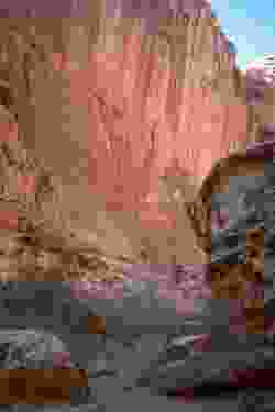
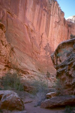 In this article, we'll study the JPEG baseline compression algorithm using the image on the right as an example. (JPEG is an acronym for "Joint Photographic Experts Group.") Some compression algorithms are lossless for they preserve all the original information. Others, such as the JPEG baseline algorithm, are lossy--some of the information is lost, but only information that is judged to be insignificant.
Before we begin, let's naively determine how much computer storage should be required for this image. First, the image is arranged in a rectangular grid of pixels whose dimensions are 250 by 375 giving a total of 93,750 pixels. The color of each pixel is determined by specifying how much of the colors red, green and blue should be mixed together. Each color component is represented as an integer between 0 and 255 and so requires one byte of computer storage. Therefore, each pixel requires three bytes of storage implying that the entire image should require 93,750  3 = 281,250 bytes. However, the JPEG image shown here is only 32,414 bytes. In other words, the image has been compressed by a factor of roughly nine.
We will describe how the image can be represented in such a small file (compressed) and how it may be reconstructed (decompressed) from this file.
The JPEG compression algorithm
First, the image is divided into 8 by 8 blocks of pixels.
Since each block is processed without reference to the others, we'll concentrate on a single block. In particular, we'll focus on the block highlighted below.
Here is the same block blown up so that the individual pixels are more apparent. Notice that there is not tremendous variation over the 8 by 8 block (though other blocks may have more).

Remember that the goal of data compression is to represent the data in a way that reveals some redundancy. We may think of the color of each pixel as represented by a three-dimensional vector (R,G,B) consisting of its red, green, and blue components. In a typical image, there is a significant amount of correlation between these components. For this reason, we will use a color space transform to produce a new vector whose components represent luminance, Y, and blue and red chrominance, Cb and Cr.
The luminance describes the brightness of the pixel while the chrominance carries information about its hue. These three quantities are typically less correlated than the (R, G, B) components. Furthermore, psychovisual experiments demonstrate that the human eye is more sensitive to luminance than chrominance, which means that we may neglect larger changes in the chrominance without affecting our perception of the image.
Since this transformation is invertible, we will be able to recover the (R,G,B) vector from the (Y, Cb, Cr) vector. This is important when we wish to reconstruct the image. (To be precise, we usually add 128 to the chrominance components so that they are represented as numbers between 0 and 255.)
When we apply this transformation to each pixel in our block
we obtain three new blocks, one corresponding to each component. These are shown below where brighter pixels correspond to larger values.
As is typical, the luminance shows more variation than the the chrominance. For this reason, greater compression ratios are sometimes achieved by assuming the chrominance values are constant on 2 by 2 blocks, thereby recording fewer of these values. For instance, the image editing software Gimp provides the following menu when saving an image as a JPEG file:
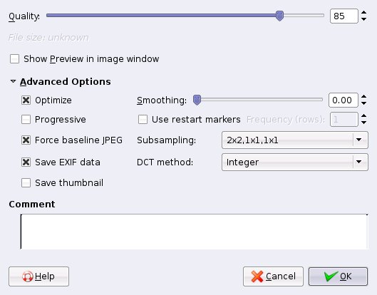
The "Subsampling" option allows the choice of various ways of subsampling the chrominance values. Also of note here is the "Quality" parameter, whose importance will become clear soon.
The Discrete Cosine Transform
Now we come to the heart of the compression algorithm. Our expectation is that, over an 8 by 8 block, the changes in the components of the (Y, Cb, Cr) vector are rather mild, as demonstrated by the example above. Instead of recording the individual values of the components, we could record, say, the average values and how much each pixel differs from this average value. In many cases, we would expect the differences from the average to be rather small and hence safely ignored. This is the essence of the Discrete Cosine Transform (DCT), which will now be explained.
We will first focus on one of the three components in one row in our block and imagine that the eight values are represented by f0, f1, ..., f7. We would like to represent these values in a way so that the variations become more apparent. For this reason, we will think of the values as given by a function fx, where x runs from 0 to 7, and write this function as a linear combination of cosine functions:
Don't worry about the factor of 1/2 in front or the constants Cw (Cw = 1 for all w except C0 =  ). What is important in this expression is that the function fx is being represented as a linear combination of cosine functions of varying frequencies with coefficients Fw. Shown below are the graphs of four of the cosine functions with corresponding frequencies w.
Of course, the cosine functions with higher frequencies demonstrate more rapid variations. Therefore, if the values fx change relatively slowly, the coefficients Fw for larger frequencies should be relatively small. We could therefore choose not to record those coefficients in an effort to reduce the file size of our image.
The DCT coefficients may be found using

Notice that this implies that the DCT is invertible. For instance, we will begin with fx and record the values Fw. When we wish to reconstruct the image, however, we will have the coefficients Fw and recompute the fx.
Rather than applying the DCT to only the rows of our blocks, we will exploit the two-dimensional nature of our image. The Discrete Cosine Transform is first applied to the rows of our block. If the image does not change too rapidly in the vertical direction, then the coefficients shouldn't either. For this reason, we may fix a value of w and apply the Discrete Cosine Transform to the collection of eight values of Fw we get from the eight rows. This results in coefficients Fw,u where w is the horizontal frequency and u represents a vertical frequency.
We store these coefficients in another 8 by 8 block as shown:
Notice that when we move down or to the right, we encounter coefficients corresponding to higher frequencies, which we expect to be less significant.
The DCT coefficients may be efficiently computed through a Fast Discrete Cosine Transform, in the same spirit that the Fast Fourier Transform efficiently computes the Discrete Fourier Transform.
Quantization
Of course, the coefficients Fw,u, are real numbers, which will be stored as integers. This means that we will need to round the coefficients; as we'll see, we do this in a way that facilitates greater compression. Rather than simply rounding the coefficients Fw,u, we will first divide by a quantizing factor and then record
round(Fw,u / Qw,u)
This allows us to emphasize certain frequencies over others. More specifically, the human eye is not particularly sensitive to rapid variations in the image. This means we may deemphasize the higher frequencies, without significantly affecting the visual quality of the image, by choosing a larger quantizing factor for higher frequencies.
Remember also that, when a JPEG file is created, the algorithm asks for a parameter to control the quality of the image and how much the image is compressed. This parameter, which we'll call q, is an integer from 1 to 100. You should think of q as being a measure of the quality of the image: higher values of q correspond to higher quality images and larger file sizes. From q, a quantity  is created using
Here is a graph of as a function of q:
Notice that higher values of q give lower values of . We then round the weights as
round(Fw,u / Qw,u)
Naturally, information will be lost through this rounding process. When either or Qw,u is increased (remember that large values of correspond to smaller values of the quality parameter q), more information is lost, and the file size decreases.
Here are typical values for Qw,u recommended by the JPEG standard. First, for the luminance coefficients:
and for the chrominance coefficients:
These values are chosen to emphasize the lower frequencies. Let's see how this works in our example. Remember that we have the following blocks of values:
Quantizing with q = 50 gives the following blocks:
The entry in the upper left corner essentially represents the average over the block. Moving to the right increases the horizontal frequency while moving down increases the vertical frequency. What is important here is that there are lots of zeroes. We now order the coefficients as shown below so that the lower frequencies appear first.
In particular, for the luminance coefficients we record
20 -7 1 -1 0 -1 1 0 0 0 0 0 0 0 -2 1 1 0 0 0 0 ... 0
Instead of recording all the zeroes, we can simply say how many appear (notice that there are even more zeroes in the chrominance weights). In this way, the sequences of DCT coefficients are greatly shortened, which is the goal of the compression algorithm. In fact, the JPEG algorithm uses extremely efficient means to encode sequences like this.
When we reconstruct the DCT coefficients, we find
| Original |
 |
 |
 |
| Reconstructed |
 |
 |
 |
| |
Y |
Cb |
Cr |
Reconstructing the image from the information is rather straightforward. The quantization matrices are stored in the file so that approximate values of the DCT coefficients may be recomputed. From here, the (Y, Cb, Cr) vector is found through the Inverse Discrete Cosine Transform. Then the (R, G, B) vector is recovered by inverting the color space transform.
Here is the reconstruction of the 8 by 8 block with the parameter q set to 50
|
 |
| Original |
Reconstructed (q = 50) |
and, below, with the quality parameter q set to 10. As expected, the higher value of the parameter q gives a higher quality image.
|
 |
| Original |
Reconstructed (q = 10) |
JPEG 2000
While the JPEG compression algorithm has been quite successful, several factors created the need for a new algorithm, two of which we will now describe.
First, the JPEG algorithm's use of the DCT leads to discontinuities at the boundaries of the 8 by 8 blocks. For instance, the color of a pixel on the edge of a block can be influenced by that of a pixel anywhere in the block, but not by an adjacent pixel in another block. This leads to blocking artifacts demonstrated by the version of our image created with the quality parameter q set to 5 (by the way, the size of this image file is only 1702 bytes) and explains why JPEG is not an ideal format for storing line art.
In addition, the JPEG algorithm allows us to recover the image at only one resolution. In some instances, it is desirable to also recover the image at lower resolutions, allowing, for instance, the image to be displayed at progressively higher resolutions while the full image is being downloaded.
To address these demands, among others, the JPEG 2000 standard was introduced in December 2000. While there are several differences between the two algorithms, we'll concentrate on the fact that JPEG 2000 uses a wavelet transform in place of the DCT.
Before we explain the wavelet transform used in JPEG 2000, we'll consider a simpler example of a wavelet transform. As before, we'll imagine that we are working with luminance-chrominance values for each pixel. The DCT worked by applying the transform to one row at a time, then transforming the columns. The wavelet transform will work in a similar way.
To this end, we imagine that we have a sequence f0, f1, ..., fn describing the values of one of the three components in a row of pixels. As before, we wish to separate rapid changes in the sequence from slower changes. To this end, we create a sequence of wavelet coefficients:
Notice that the even coefficients record the average of two successive values--we call this the low pass band since information about high frequency changes is lost--while the odd coefficients record the difference in two successive values--we call this the high pass band as high frequency information is passed on. The number of low pass coefficients is half the number of values in the original sequence (as is the number of high pass coefficients).
It is important to note that we may recover the original f values from the wavelet coefficients, as we'll need to do when reconstructing the image:
We reorder the wavelet coefficients by listing the low pass coefficients first followed by the high pass coefficients. Just as with the 2-dimensional DCT, we may now apply the same operation to transform the wavelet coefficients vertically. This results in a 2-dimensional grid of wavelet coefficients divided into four blocks by the low and high pass bands:
As before, we use the fact that the human eye is less sensitive to rapid variations to deemphasize the rapid changes seen with the high pass coefficients through a quantization process analagous to that seen in the JPEG algorithm. Notice that the LL region is obtained by averaging the values in a 2 by 2 block and so represents a lower resolution version of the image.
In practice, our image is broken into tiles, usually of size 64 by 64. The reason for choosing a power of 2 will be apparent soon. We'll demonstrate using our image with the tile indicated. (This tile is 128 by 128 so that it may be more easily seen on this page.)
Notice that, if we transmit the coefficients in the LL region first, we could reconstruct the image at a lower resolution before all the coefficients had arrived, one of aims of the JPEG 2000 algorithm.
We may now perform the same operation on the lower resolution image in the LL region thereby obtaining images of lower and lower resolution.
The wavelet coefficients may be computed through a lifting process like this:
The advantage is that the coefficients may be computed without using additional computer memory--a0 first replaces f0 and then a1 replaces f1. Also, in the wavelet transforms that are used in the JPEG 2000 algorithm, the lifting process enables faster computation of the coefficients.
The JPEG 2000 wavelet transform
The wavelet transform described above, though similar in spirit, is simpler than the ones proposed in the JPEG 2000 standard. For instance, it is desirable to average over more than two successive values to obtain greater continuity in the reconstructed image and thus avoid phenomena like blocking artifacts. One of the wavelet transforms used is the Le Gall (5,3) spline in which the low pass (even) and high pass (odd) coefficients are computed by
As before, this transform is invertible, and there is a lifting scheme for performing it efficiently. Another wavelet transform included in the standard is the Cohen-Daubechies-Fauraue 9/7 biorthogonal transform, whose details are a little more complicated to describe though a simple lifting recipe exists to implement it.
It is worthwhile to compare JPEG and JPEG 2000. Generally speaking, the two algorithms have similar compression ratios, though JPEG 2000 requires more computational effort to reconstruct the image. JPEG 2000 images do not show the blocking artifacts present in JPEG images at high compression ratios but rather become more blurred with increased compression. JPEG 2000 images are often judged by humans to be of a higher quality.
At this time, JPEG 2000 is not widely supported by web browsers but is used in digital cameras and medical imagery. There is also a related standard, Motion JPEG 2000, used in the digital film industry.
References
- Home pages for the JPEG committee and JPEG 2000 committee
- Tinku Archarya, Ping-Sing Tsai, JPEG2000 Standard for Image Compression: Concepts, Algorithms and VLSI Architectures, Wiley, Hoboken. 2005.
- Jin Li, Image Compression: The mathematics of JPEG 2000, Modern Signal Processing, Volume 46, 2003.
- Ingrid Daubechies, Ten lectures on wavelets, SIAM, Philadelphia. 1992.
- K.R. Rao, Patrick Yip, Discrete Cosine Transform: Algorithms, Advantages, Applications, Academic Press, San Diego. 1990.
- Wikipedia entries for JPEG and JPEG 2000.
David Austin
Grand Valley State University
david at merganser.math.gvsu.edu
Those who can access JSTOR can find some of the papers mentioned above there. For those with access, the American Mathematical Society's MathSciNet can be used to get additional bibliographic information and reviews of some these materials. Some of the items above can be accessed via the ACM Portal , which also provides bibliographic services.


