The Mathematics Behind Quantum Computing: Part I
Posted May 2007.
This column and next month's will present a description of Shor's Factorization Algorithm in terms appropriate for a general mathematical audience...
Tony Phillips
Stony Brook University
tony at math.sunysb.edu
Quantum computing
Quantum computing may be just around the corner or it may be, for all practical purposes, permanently out of reach: The physics needed for a useful quantum computer has not yet been discovered, and may in fact not exist.
A quantum computer, real or potential, is essentially different from an adding machine. Whereas the dials in Pascal's A.D. 1645 brass calculator always line up to read out exactly one 6-digit number, the set of qubits in a quantum register exist in a superposition of states: When the register is interrogated one of these states is read out, with a definite probability, and the remaining information is lost. Because the register can simultaneously be "in" a huge number of states, a huge number of calculations may be carried out simultaneously. But the inputs to a quantum computer must be organized to take advantage of superposition, and the calculating process must force the probabilistic output to give useful information. This is the problem of programming a quantum computer, and in certain important and interesting cases it has been solved. One of the quantum computing algorithms, a factorization algorithm due to Peter Shor, will be the focus of these two columns.
The factorization problem
Communication security today is almost universally ensured by the use of RSA encryption. This method relies on the inaccessibility of large prime factors of a large composite number. The problem is an artificial one: The encrypter takes two (or more) large primes and multiplies them. The decrypter tries to work backwards from the product to the factors. It is hard work. The largest number factored so far ("RSA-640") had 193 decimal digits and took "approximately 30 2.2GHz-Opteron-CPU years," over five months of calendar time. At that rate a 1024-bit number, the size currently recommended by a commercial cryptology site, would take on the order of 10145 years ("bit" is short for "binary digit;" each additional bit contributes a factor of 2 to the size of the calculation). The site adds: "For more security or if you are paranoid, use 2048 or even 4096 bits."
A quantum computer of suitable size could factor these large numbers in a much shorter time. For a 1024-bit number, Shor's Algorithm requires on the order of 10243, about one billion, operations. I do not have any information on how quickly quantum operations can be executed, but if each one took one second our factorization would last 34 years. If a quantum computer could run at the speed of today's electronic computers (100 million instructions per second and up) then factorization of the 1024-bit number would be a matter of seconds.
A note on "suitable size." To run Shor's Algorithm on a 1024-bit number requires two quantum registers, one of 2048 qubits and one of 1024. These qubits all have to be "in coherence," so that the totality of their states behaves as a single, entangled state. (More about entanglement later). It was reported as an extraordinary technical feat when IBM scientists in 2001 constructed a coherent quantum register with 7 qubits and used it with Shor's Algorithm to factor 15.
This column and next month's will present a description of Shor's Factorization Algorithm in terms appropriate for a general mathematical audience. This month will cover the number-theoretical underpinning along with the Discrete and Fast Fourier Transforms. These convert factorization into a frequency-detection problem which is structured so that it can be adapted for quantum computation. The problem itself has a definite answer but takes exponential time to get there. Next month's column will address the more specifically quantum-computational aspects of the algorithm, including superposition and entanglement, leading up to Shor's ingenious quantum jiu-jitsu, which forces the quantum read-out, with high probability, to give a useful answer. That probability is high enough, and the running time on a suitable machine would be short enough, for the calculation to be repeated until the unknown factors are produced.
Number Theory and Fourier Analysis
{C}
The light from a star can be split into a spectrum, where the characteristic frequencies of its elements can be detected. Analogously, a composite number N can be made to generate a spectrum, from which its factors can be calculated.
Choose a number a relatively prime to N, and make the list of integer powers of a modulo N: a, a2, a3, ... . If a and N are relatively prime, it follows from a theorem of Euler that this list will eventually include the number 1. (Euler's Theorem says specifically that if φ(N) denotes the number of positive integers less that N which are coprime to N then aφ(N) is congruent to 1 modulo N). Suppose this happens for an even power of a, say a2b = 1 mod N, i.e. a2b – 1 = 0 mod N. This means that (ab + 1) (ab – 1) is a multiple of N; if it is one times N we have our factors; otherwise the Euclidean Algorithm will speedily find a common factor of, say, ab + 1 and N.
These examples are trivially simple, but illustrate the phenomenon:
- Take N = 85 and a = 19. The powers of 19 mod 85 are 19, 21, 59, 16, 49, 81, 9, 1, 19, 21, ...; in particular 198 = 1 mod 85. We deduce that 194 + 1 = 17 and 194 – 1 = 15 both have common factors with 85. In fact the first is a factor and the second has 5 as common divisor with 85.
- Take N = 85 and a = 33. The powers of 33 mod 85 are 33, 69, 67, 1, 33, 69, 67, 1, ...; in particular 334 = 1 mod 85. We deduce that 332 + 1 = 70 and 332 – 1 = 68 both have common factors with 85. In fact the first yields 5 and the second 17.
- Note that φ(85) = 64, so 64 would always work; but this number cannot be calculated a priori: you have to know the prime factorization 85 = 17 x 5, and use the rule φ(pq) = (p–1)(q–1) for p and q prime.
How do we get our hands on b? Just examining the terms of the sequence and waiting for 1 to show up takes too long, because the length of the list is commensurate with the number N we want to factor: It increases exponentially with the number, say n, of bits used to write N. But think of the stream of numbers a mod N, a2 mod N, a3 mod N, ... as the light emitted by N. If we can find the frequency, or equivalently the period, with which this sequence repeats itself, we can use the equivalence aj = ak <=> aj–k = 1 (modulo N), and find a factorization of N as above. We will see that on a quantum computer, this computation requires a number of steps increasing only as a polynomial in n. That is the key to quantum factorization.
Discrete Fourier Transforms
Fourier transforms detect periodicity; we will find b using a quantum adaptation of the Fast Fourier Transform, a speeded-up version of the Discrete Fourier Transform, which itself arises from adapting to sequences the Fourier Series designed to work with continuous functions.
The (complex) Fourier coefficients of a real-valued function f(x) defined on [0,2A] are
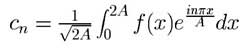 .
.
Notes:
- Writing ei nπx/A as cos nπx/A + i sin nπx/A and cn = an + i bn gives the usual sine and cosine coefficients, except that c0 is twice the usual a0.
- The factor 1/
 allows the identity
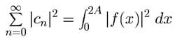 ,
,
which will be important in our later quantum computations.
Suppose now we think of a sequence f = f0, f1, ... , f2A–1 (A now an integer), as the set of values at x = 0, x = 1, x = 2, ... , x = 2A–1 of a function f(x) defined on the interval [0,2A], and that we define a new cn by replacing the Fourier integral with a left-hand sum with 2A equal subdivisions of length 1. This sum only involves the elements of f:
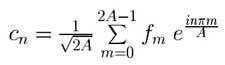 .
.
Notes:
- ei (2A+k)mπ/A = ei 2mπ ei kmπ/A = ei kmπ/A, so coefficients indexed 2A and higher give no extra information.
- The sequence c of coefficients c0, ... , c2A–1 is the Discrete Fourier Transform of the sequence f.
- Essentially the same calculation retrieves f from c:
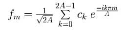
(note the minus sign in the exponents).
Transform of a periodic sequence
Suppose that f has period p, i.e. fm+p = fm for every value of m; the simplest case to analyze is when p is a divisor of 2A, say p = 2A/k, k an integer. In that case, if n is not a multiple of k (green boxes in the examples below) the periodic reappearances of a sequence item fm are multiplied by coefficients which cycle through a complete set of roots of 1, and thereby add up to zero. The explicit formula is:
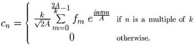
So the only chance for a non-zero Fourier coefficient is when n is a multiple of k, (and then, up to a factor, c0, ck, c2k, ... , c(p–1)k are the 0th, 1st, 2nd, ... , (p–1)-st Fourier coefficients of the sequence f restricted to a single period).
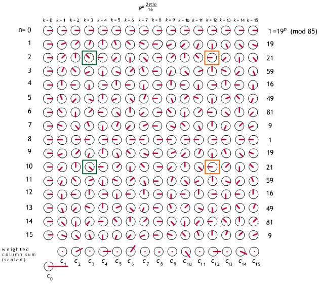
Fig. 1. Discrete Fourier Transform analysis of the sequence given by the first 16 powers of 19 (modulo 85), a sequence with period 8 and frequency 16/8 = 2. When n is a multiple of 2 (e.g. orange boxes) every re-occurrence of a sequence item gets the same coefficient, and cn has a chance of being nonzero. Otherwise (e.g. green boxes) it is zero. The complex numbers in the matrix are graphically represented as unit vectors. Each cn is the weighted vector sum of the entries in the column above it, weights coming from the fk column on the right, with an overall factor of 1/ = 1/4. The cn have been uniformly scaled to fit in the picture.
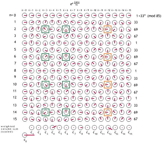
Fig. 2. Discrete Fourier Transform analysis of the sequence given by the first 16 powers of 33 (modulo 85). This sequence has period 4 and frequency 16/4=4. The non-zero cn only occur for n a multiple of 4. Graphic conventions are the same as in Fig. 1.
Why powers of 2?
I have chosen for illustration a number (85) which generates power residue sequences with periods which are powers of 2, and I have chosen to analyze a length (16) of sequence which is also a power of 2. The second choice is not immaterial: The Fast Fourier Transform we will use, and its quantum adaptation, both require it. The first choice is only for covenience in generating a small example. Shor shows that to get a reliable read on the power residue period in general, in the problem of factoring N, one must analyze sequences of a length 2n between N2 and 2N2. So to analyze a number like 85 realistically, we would have to work with sequences of length 8192.
The Fast Fourier Transform
The Fast Fourier Transform which adapts directly to quantum computation is the Radix-2 Cooley-Tukey algorithm, invented in 1965 (reinvented, actually, since it later turned out to have been known to Gauss). To control the width of this presentation, I am going to work with the order-8 Discrete Fourier Transform, rather than order-16 as above. Taking ω = eiπ/4= 2–1/2(1 + i) as our primitive 8th root of 1, the 0-7th powers of ω are
1, eiπ/4, eiπ/2, e3iπ/4, eiπ, e5iπ/4, e3iπ/2, e7iπ/4,
or
1, ω, i, iω, –1, –ω, –i, –iω,
the numbers represented graphically above as
 ,
,  ,
,  ,
,  ,
,  ,
,  ,
,  ,
,  .
.
The transform c of an arbitrary length-8 sequence f = f0, f1, ..., f7, given by
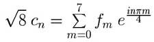 ,
,
would be produced from the array
| |
|
|
|
|
|
|
|
|
| 1 |
1 |
1 |
1 |
1 |
1 |
1 |
1 |
f0 |
| 1 |
ω |
i |
iω |
–1 |
–ω |
–i |
–iω |
f1 |
| 1 |
i |
–1 |
–i |
1 |
i |
–1 |
–i |
f2 |
| 1 |
iω |
–i |
ω |
–1 |
–iω |
i |
–ω |
f3 |
| 1 |
–1 |
1 |
–1 |
1 |
–1 |
1 |
–1 |
f4 |
| 1 |
–ω |
i |
–iω |
–1 |
ω |
–i |
iω |
f5 |
| 1 |
–i |
–1 |
i |
1 |
–i |
1 |
i |
f6 |
| 1 |
–iω |
–i |
–ω |
–1 |
iω |
i |
ω |
f7 |
| c0 |
c1 |
c2 |
c3 |
c4 |
c5 |
c6 |
c7 |
|
by setting the last row to be f0 times the first plus ... plus f7 times the eighth, the whole sum divided by  . This calculation would require eight multiplications and seven additions for each item in c, or 120 operations in all. Working with a sequence of length 2n, the number of operations would be 2n (2n+1 – 1).
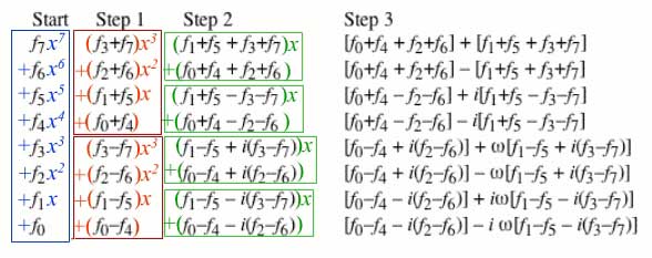
Our Fast Fourier Transform leads in n steps from the elements f0, ... f2n–1 of the input sequence to the coefficients c0, ... c2n–1 of its Discrete Fourier Transform. We illustrate the process here for n = 3. Each column represents a successive step of the calculation.
Line
0
1
2
3
4
5
6
7 |
Start
f7
f6
f5
f4
f3
f2
f1
f0 |
Step 1
f3+f7
f2+f6
f1+f5
f0+f4
f3–f7
f2–f6
f1–f5
f0–f4 |
Step 2
f1+f5 + f3+f7
f0+f4 + f2+f6
f1+f5 – f3–f7
f0+f4 – f2–f6
f1–f5 + i(f3–f7)
f0–f4 + i(f2–f6)
f1–f5 – i(f3–f7)
f0–f4 – i(f2–f6) |
Step 3
[f0+f4 + f2+f6] + [f1+f5 + f3+f7]
[f0+f4 + f2+f6] – [f1+f5 + f3+f7]
[f0+f4 – f2–f6] + i[f1+f5 – f3–f7]
[f0+f4 – f2–f6] – i[f1+f5 – f3–f7]
[f0–f4 + i(f2–f6)] + ω[f1–f5 + i(f3–f7)]
[f0–f4 + i(f2–f6)] – ω[f1–f5 + i(f3–f7)]
[f0–f4 – i(f2–f6)] + iω[f1–f5 – i(f3–f7)]
[f0–f4 – i(f2–f6)] – i ω[f1–f5 – i(f3–f7)] |
= c0
= c4
= c2
= c6
= c1
= c5
= c3
= c7 |
Notes:
- In this presentation of the algorithm the elements of the sequence f are ordered backwards and the elements of the transformed sequence c appear in "bit reversed" order: cn appears on line k where (in binary) k is n written backwards; e.g. c6 (110) appears on line 3 (011).
- Working with a sequence of length 2n the computation table has 2n rows; in each row are n columns requiring computation; each entry is calculated as a linear combination of two entries from the previous column, and so requires two multiplications and a sum; altogether 3n operations per row for a total of 3n2n operations. Contrasting this with the 2n (2n+1 – 1) operations to implement the Discrete Fourier Transform shows that the Fast Fourier Transform is fast indeed.
Why does this work?
The most transparent explanation I know uses properties of polynomial long division. Here I will specalize to the example at hand.
we can understand Step 1 as transforming the degree-7 polynomial f into two degree-3 polynomials (red boxes) each of which can produce, via its remainders, half of the cn. Then Step 2 transforms each of the degree-3 polynomials into two degree-1 polynomials (green boxes), each of which can produce a quarter of the cn, and Step 3 transforms each of the degree-1 polynomials into two degree-0 polynomials, which are their own remainders.
- For a sequence f of length 8, the expression for the nth Fourier coefficient can be read as the value at einπ/4 of the polynomial f(x) = f0 + f1 x + ... + f7 x7:
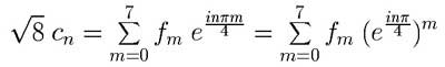 .
.
- If a polynomial p(x) is divided by the monic, first degree polynomial x–a, the remainder is exactly the number p(a).
- So cn is (1/) times the remainder when f(x) is divided by (x– einπ/4). The shift in focus from evaluation of a polynomial to calculation of remainders is the key to the economies of the Fast Fourier Transform.
- The remainder when f(x) is divided by x4– 1 is
(f3 + f7)x3 + (f2 + f6)x2 + (f1 + f5)x + (f0 + f4),
and its remainder upon division by x4+ 1 is
(f3 – f7)x3 + (f2 – f6)x2 + (f1 – f5)x + (f0 – f4).
And in general, if a2n–1x2n–1 + ... + a0 is divided by xn – c, the remainder is an–1xn–1 + ... + a0 + c (a2n–1xn–1 + ... + an) [Note: last term corrected (from a2n ) 6/2/14]. This is what makes calculation of remainders especially simple when the overall degree is a power of 2.
- Since
x4 – 1 = (x2 – 1)(x2 + 1) = (x – 1)(x + 1)(x – i)(x + i),
it follows that f(x) and p(x) = (f3 + f7)x3 + (f2 + f6)x2 + (f1 + f5)x + (f0 + f4) have the same remainder when divided by any one of the factors (x – 1), (x + 1), (x – i) or (x + i).
- Because if f(x) = (x4 – 1) q(x) + p(x) and for example p(x) = (x – i)q'(x) + a, then f(x) = [(x – 1)(x + 1) (x – i)(x + i)]q(x) + (x – i)q'(x) + a also has remainder a when divided by (x – i).
- Similarly, since x4 + 1 = (x2 – i)(x2 + i) = (x – ω)(x + ω) (x – iω)(x + iω), the degree-3 polynomial (f3 – f7)x3 + (f2 – f6)x2 + (f1 – f5)x + (f0 – f4) can be used, via its remainders, to calculate f(ω), etc.
- Returning to the Fast Fourier Transform calculation
The mathematics behind quantum computing will be continued in next month's Feature Column.
References
{C}
For the Fast Fourier Transform, I have followed Henry Laufer's text Discrete Mathematics and Applied Modern Algebra, Prindle, Weber & Schmidt, Boston 1984.
The Wikipedia entry on Fast Fourier Transform gives an alternative explanation; it also provides references to Cooley and Tukey's 1965 paper as well as to the spot in Gauss' Nachlass where he develops the technique, both items in its extensive bibliography on the ancient and recent history of the algorithm.
References on the "Quantum Fourier Transform" and on Shor's Algorithm:
D. Coppersmith, An Approximate Fourier Transform Useful in Quantum Factoring, IBM Research Report 07/12/94, available as arXiv:quant-ph/0201067.
A. Ekert and R. Jozsa, Quantum computation and Shor's factoring algorithm, Reviews of Modern Physics 68 (1996) 733-753
Peter W. Shor, Algorithms for Quantum Computation: In: Proceedings, 35th Annual Symposium on Foundations of Computer Science, Santa Fe, NM, November 20--22, 1994, IEEE Computer Society Press, pp. 124--134. An expanded version is available, under the title
Polynomial-Time Algorithms for Prime Factorization and Discrete Logarithms on a Quantum Computer, as arXiv:quant-ph/9508027.
Tony Phillips
Stony Brook University
tony at math.sunysb.edu
Those who can access JSTOR can find some of the papers mentioned above there. For those with access, the American Mathematical Society's MathSciNet can be used to get additional bibliographic information and reviews of some these materials. Some of the items above can be accessed via the ACM Portal , which also provides bibliographic services.


