Algebraic and Analytic Compactifications of Moduli Spaces

The Tour Ahead

The basic objects of algebraic geometry, such as subvarieties of a projective space, are defined by polynomial equations. The seemingly innocuous observation that one can vary the coefficients of these equations leads at once to unexpectedly deep questions:

•

When are objects with distinct coefficients equivalent?

•

What types of geometric objects appear if those coefficients move “towards infinity”?

•

Can we make sense of “equivalence classes at infinity”?

Searching for answers leads to the discovery of moduli spaces and their compactifications, parametrizing equivalence classes of said objects.

The construction of compact moduli spaces and the study of their geometry amounts nowadays to a busy and central neighborhood of algebraic geometry. Any vibrant district in an old city, of course, has too many landmarks to visit, and the first job of a tour guide is to curate a selection of sites and routes — including multiple routes to the same site for the different perspectives they afford. Our tour today has three main stops: elliptic curves, Picard curves (together with “points on a line,” their alter ego), and a brief panoramic glimpse of the general theory.

As for the routes, we first approach the elliptic curve example along the unswerving path that compactifies algebro-geometric moduli spaces with “limiting” algebro-geometric invariants. The way is straight, but entails scaling a brick wall to discover what is meant by “limits.” Our subsequent turn down 19th-century vennels will unveil a connection as old as algebraic geometry itself: associated to our algebraic varieties are analytic periods, producing a period map from our moduli space to a classifying space for periods. While lacking the ideological consistency of the former route, the “limits” of this one are more conceptually straightforward — with Calculus providing a door in the wall.

For the Picard curve example, we reverse the order of these two approaches; this example is important because it is the simplest one where there are multiple natural compactifications of both sorts. Both examples have two very nice features, besides involving objects one can draw on paper. First, the period map is close to being an isomorphism and is inverted by modular forms, an observation going back in the elliptic case to work of Weierstraß. Second, the period map extends to isomorphisms of the various algebraic and analytic compactifications.

These examples will illustrate techniques and methods in moduli theory, preparing the stage for our last stop, high above the city. From there we shall be able to see a vague outline of the modern definition of moduli spaces, as well as various algebro-geometric (GIT, KSBA, K-stable) and Hodge-theoretic (Baily-Borel, toroidal, etc.) compactifications of the same moduli space. The aim of our brief journey is to travel towards understanding their differences — and especially their spectacular coincidences.

1. Elliptic Curves

With a rich history going back to Abel, Jacobi, and Weierstraß in their guise as complex 1-tori (think of the surface of a donut), elliptic curves are central objects in many areas of mathematics, from cryptography to complex analysis. At this first stop on our tour, we’ll use their moduli space to illustrate constructions such as geometric quotients and the period map (and its inversion).

1.1. Algebraic perspective

Our starting point is the fact, first hinted at by Jacobi in 1834, that any complex 1-torus can be realized as a smooth plane cubic — that is, an algebraic curve defined as the zero-locus in $(\mathbb{C})\mathbb{P}^2$ of a homogeneous polynomial of degree three in 3 variables

$$\begin{equation*} F(x_0,x_1,x_2) = a_{300}x_0^3 + \cdots + a_{012}x_1x_2^2 + a_{003}x_2^3, \end{equation*}$$

with certain conditions on the coefficients to guarantee the smoothness of $\{F(x_0,x_1,x_2)=0\}$. Conversely, for an algebraic geometer, it is natural to approach the set of elliptic curves via a suitable quotient of the set of all such cubics.

Without the smoothness requirement, the coefficients of such equations comprise all ordered 10-tuples of complex numbers $[a_{300}{:} a_{210}{:} \cdots {:} a_{012}{:} a_{003}]$, not all zero, defined up to scaling (by $\mathbb{C}^{\times }$). Since an equation $F(x_0,x_1,x_2)=0$ is determined uniquely by its coefficients up to scaling, we conclude that the set of all plane cubics can be identified with the set of complex points of the projective space $\mathbb{P}^{9}$. (Outside the open set parametrizing smooth cubics, there are $8$ different flavors of singular cubics as displayed in Figure 1.)

Figure 1.

Classification of plane cubics.

The fact that the set of all plane cubics is itself a complex algebraic variety is not a coincidence! Instead, it is our first encounter with one of the most important objects in moduli theory: the Hilbert scheme. Indeed, to keep track of the complex solutions of polynomial equations within projective space, we need to fix an invariant known as the Hilbert polynomial. This polynomial records geometric information about our solutions such as their dimension and degree. It was shown in 1961 by Grothendieck that there exists an algebro-geometric space (that is, a projective scheme) $\operatorname {Hilb}^{p(m)}_r$ which parametrizes all the closed complex solutions of polynomial equations in $\mathbb{P}^r$ with Hilbert polynomial $p(m)$. In our particular example, all plane cubics have Hilbert polynomial equal to $p(m)=3m$, and the associated Hilbert scheme is $\mathbb{P}^9$. Every point in $\mathbb{P}^9$ corresponds to a curve with this Hilbert polynomial and vice versa.

At this juncture the reader will point out that $\mathbb{P}^9$ is certainly not the sought-for “moduli space of elliptic curves,” because it includes singular cubics. But the open subset parametrizing smooth cubics is not the solution either. The reason is that given an elliptic curve defined by the equation $\{ F(x_0,x_1,x_2) = 0 \}$, we can use an invertible linear change of coordinates $x_i \mapsto a_{i0}x_0 + a_{i1}x_1 + a_{i2}x_2$ with $a_{ij} \in \mathbb{C}$, to obtain another equation $\{G(x_0, x_1, x_2) = 0 \}$. The elliptic curve defined by this second equation is isomorphic as a complex variety to the first one, and yet the Hilbert scheme tells us that they are different objects.

The critical observation here is that if we are parametrizing varieties $X \subset \mathbb{P}^n$ with a fixed Hilbert polynomial, then we want to account for the automorphisms of the ambient projective space. In our example the ambient space of elliptic curves $\{F(x_0, x_1, x_2) =0 \}$ is $\mathbb{P}^2$ and the group $\operatorname {SL}_3(\mathbb{C})$ associated to linear automorphisms $x_i \mapsto a_{i0}x_0 + a_{i1}x_1 + a_{i2}x_2$ has dimension 8. Therefore, of the 9 degrees of freedom associated with the coefficients of the equation $F(x_0,x_1,x_2)$, only one is intrinsic to the geometry of the elliptic curve, while the other eight are related to linear changes of coordinates in the ambient space.

The relation between elliptic curves and $\operatorname {SL}_3(\mathbb{C})$-orbits is tight; two plane cubics $\{ F(x_0,x_1,x_2) = 0\}$ and $\{ G(x_0,x_1,x_2)=0 \}$ represent isomorphic elliptic curves (algebraically or complex analytically) if and only if $g \cdot F(x_0,x_1,x_2) = G(x_0,x_1,x_2)$ for some $g\in \operatorname {SL}_3(\mathbb{C})$. Therefore, the set of elliptic curves up to isomorphism can be identified with $\operatorname {SL}_3(\mathbb{C})$-orbits of smooth plane cubics. Although the set of such orbits exists as a topological space, it is not at all obvious that this space is itself a complex variety. We arrive at one of the most delicate problems in algebraic geometry: Given the action of a linear group $G$ on a variety $X$, does there exist an algebro-geometric space parametrizing the $G$-orbits in $X$?

The correct framework for constructing quotients within algebraic geometry is given by Geometric Invariant Theory (GIT), initiated by Mumford in 1969 17. One of the key results from GIT is the existence of an open locus $\mathcal{U}^{s} \subset X$ called the stable locus and a well-defined geometric quotient, which in our case is

$$\begin{equation*} \mathbf{M}_{1,1} \coloneq \mathcal{U}^s/\operatorname {SL}_3(\mathbb{C}) \cong \mathbb{C}. \end{equation*}$$

One of the first exercises in GIT is to show that $\mathcal{U}^s$ is the locus parametrizing smooth plane cubics, see 17, Example 7.12. The fact that the quotient is geometric means that every point of $\mathbf{M}_{1,1}$ corresponds to a unique $\operatorname {SL}_3(\mathbb{C})$-orbit of a smooth cubic. Therefore, we arrive at our first (and almost correct!) example of a moduli space: $\mathbf{M}_{1,1}$ is the “moduli space” of elliptic curves up to isomorphism.

We also arrive at the crux of our problem: $\mathbf{M}_{1,1}$ is a non-compact variety. Is there a natural compact (projective) variety that contains it and that parametrizes a larger class of algebraic varieties? It will be tempting to consider a naive quotient of $\mathbb{P}^9$ by $\operatorname {SL}_3(\mathbb{C})$ for constructing a compactification of $\mathbf{M}_{1,1}$. However, these naive quotients are usually either of the wrong dimension or yield a non-Hausdorff topological space. Here we use a second key result from GIT: There exists a (usually larger) open set $\mathcal{U}^{ss}$, called the semistable locus, containing $\mathcal{U}^{s}$ and admitting a well-defined “categorical quotient.” In our case this is

$$\begin{equation*} \overline{\mathbf{M}}_{1,1}^{\mathrm{GIT}} \coloneq \mathcal{U}^{ss} \sslash \operatorname {SL}_3(\mathbb{C}) \cong \mathbb{P}^1, \end{equation*}$$

a complex projective variety compactifying $\mathbf{M}_{1,1}$.

To understand the geometry of the above compactification, we recall that $\mathbb{P}^9$ parametrizes all possible plane cubics. This includes our large open set $\mathcal{U}^s$ parametrizing the smooth plane cubics and smaller loci parametrizing degenerations such as nodal cubics, the union of a conic and a line, etc. It is a non trivial fact that our semistable locus $\mathcal{U}^{ss}$ parametrizes all curves with at worst a singularity locally of the form $\{ xy=0\}$; these curves are represented at the top left section of Figure 1.

The categorical quotient is not the naive one: the points of $\overline{\mathbf{M}}_{1,1}^{\mathrm{GIT}}$ are not in bijection with the $\operatorname {SL}_3(\mathbb{C})$-orbits of curves parametrized by the semistable locus $\mathcal{U}^{ss}$. Indeed, all of the orbits within the eight-dimensional locus $\mathcal{U}^{ss} \setminus \mathcal{U}^s$ are identified with a single point in $\overline{\mathbf{M}}_{1,1}^{\mathrm{GIT}}$ even though they represent non-isomorphic curves. However, there is a unique “minimal closed” $\operatorname {SL}_3(\mathbb{C})$-orbit associated to the point $\overline{\mathbf{M}}_{1,1}^{\mathrm{GIT}} \setminus \mathbf{M}_{1,1}$: namely, the orbit of the “triangle” cubic $\{ x_0x_1x_2=0 \}$.

1.2. Analytic perspective

Turning to a complex-analytic perspective, we recall that an elliptic curve $C$ can be viewed as the cartesian product of two circles $S^1 \times S^1$ with a complex structure. By considering these two circles we obtain a homology basis $\alpha ,\beta \in H_1(C,\mathbb{Z})$ (oriented so that $\alpha \cdot \beta =1$).

Up to scale, there is a unique holomorphic form $\omega \in \Omega ^1(C)$, with period ratio $\tau \coloneq {\int _{\beta }\omega }/{\int _{\alpha }\omega }$ in the upper-half plane $\mathfrak{H}$. This $\tau$ is well-defined modulo the action of $\gamma =\left(\begin{smallmatrix} a&b\\ c&d\end{smallmatrix}\right)\in \Gamma =\operatorname {SL}_2(\mathbb{Z})$ through fractional-linear transformations $\gamma (\tau )=\tfrac{a\tau +b}{c\tau +d}$ induced by changing the homology basis. We claim that the resulting (analytic) invariant $[\tau ]\in \mathfrak{H}/\Gamma$ captures the (algebraic) isomorphism class of $C$.

This is closely related to the classical theory of modular forms. Here “modular” refers to the moduli of complex 1-tori $\mathbb{C}/\Lambda$, or equivalently of the lattice $\Lambda$; and the “forms” are essentially functions on this moduli space (i.e., of the lattice $\Lambda$) with certain transformation properties depending on a weight $k\in \mathbb{N}$. The (biperiodic) Weierstraß $\wp$-function associated to the lattice $\Lambda =\mathbb{Z}\langle 1,\tau \rangle$,

$$\begin{equation*} \wp (u)\coloneq u^{-2}+\sum _{\lambda \in \Lambda \setminus 0}[(u+\lambda )^{-2}-\lambda ^{-2}], \end{equation*}$$

satisfies $(\wp ')^2=4\wp ^3-g_2(\tau )\wp -g_3(\tau )$, where $g_2(\tau )\coloneq 60\sum _{\lambda \in \Lambda \setminus 0}\lambda ^{-4}$ and $g_3(\tau )\coloneq 140\sum _{\lambda \in \Lambda \setminus 0}\lambda ^{-6}$ are modular forms $M_k(\Gamma )$ of weights $k=4$ resp. $6$. That is, they transform by the automorphy factor $(c\tau +d)^k$ under pullback by $\gamma \in \Gamma$, which makes $\pmb{\jmath }\coloneq \tfrac{g_2^3}{g_2^3-27g_3^2}\colon \mathfrak{H}/\Gamma \to \mathbb{C}$ into a well-defined function. Evidently, the image $E_{\tau }$ of the map $W\colon \mathbb{C}/\Lambda \hookrightarrow \mathbb{P}^2$ sending $u\mapsto [1:\wp (u):\wp '(u)]$ is a Weierstraß cubic

$$\begin{equation} X_2^2X_0=4X_1^3-g_2 X_1 X_0^2-g_3 X_0^3=4\prod _{i=1}^3(X_1-e_i X_0), \tag{1}{} \end{equation}$$

with period ratio $\tau$.

The key point is that any $C$ can be brought into this form (without changing $[\tau ]$) through the action of $\operatorname {SL}_3(\mathbb{C})$ on coordinates. Fix a flex point $o\in C$ (i.e., $(C\cdot T_o C)=3$); since the dual curve $\check{C}$ has degree $6$, there are 3 more tangent lines $\{T_{p_i}C\}_{i=1}^3$ passing through $o$. The $\{p_i\}$ are collinear, since otherwise one could construct a degree-1 map $C\to \mathbb{P}^1$. So we may choose coordinates to have $o=[0{:}0{:}1]$, $T_o C=\{X_0=0\}$, $\{X_2=0\}\cdot C=\sum _{i=1}^3 p_i$, and $\sum _{i=1}^3\tfrac{X_1}{X_0}(p_i)=0$, which puts us in the above form 1. In fact, if $\jmath \coloneq \pmb{\jmath }(\tau )\notin \{0,1,\infty \}\eqcolon \Sigma$, then rescaling yields a member of the family

$$\begin{equation} y^2=4x^3-\tfrac{27\jmath }{\jmath -1}x-\tfrac{27\jmath }{\jmath -1} \tag{2}{} \end{equation}$$

over $\mathbb{P}^1\setminus \Sigma$, whose period map $[\tau ]\colon \mathbb{P}^1\setminus \Sigma \to \mathfrak{H}/\Gamma$ composed with $\pmb{\jmath }$ extends to the identity $\mathbb{C}\to \mathbb{C}$. Hence $C\underset{\mathrm{SL}_3}{\cong }C'$ $\implies$ $[\tau ]=[\tau ']$ $\implies$ $\jmath =\jmath '$ $\implies$ $C\underset{\mathrm{SL}_3}{\cong }C'$ yields the claimed equivalence of analytic and algebraic “moduli,” and $\pmb{\jmath }$ is an isomorphism.

While the choice of $o$ does not refine the moduli problem, keeping track of the ordered 2-torsion subgroup $\{o,p_1,p_2,p_3\}$ does. In 1, this preserves the ordering of the $\{e_i\}$, which are parametrized by the weight-2 modular forms $\wp (\tfrac{1}{2}),\wp (\tfrac{\tau }{2}),\wp (\tfrac{\tau +1}{2})$ with respect to $\Gamma (2)\coloneq \ker \{\Gamma \to \mathrm{SL}_2(\mathbb{Z}/2\mathbb{Z})\}$. The roles of $\pmb{\jmath }$ and 2 are played by $\mathbfscr{l}\coloneq \tfrac{e_3-e_2}{e_1-e_2}\colon \mathfrak{H}/\Gamma (2)\overset{\cong }{\to }\mathbb{P}^1\setminus \Sigma$ and the Legendre family $y^2=x(x-1)(x-\ell )$, with $\pmb{\jmath }=\tfrac{4}{27}\tfrac{(1-\mathbfscr{l}-\mathbfscr{l}^2)^3}{\mathbfscr{l}^2 (1-\mathbfscr{l})^2}$ describing the 6:1 covering $\mathfrak{H}/\Gamma (2)\twoheadrightarrow \mathfrak{H}/\Gamma$. Notice that $\ell$ parametrizes the cross-ratio of 4 (ordered) points on $\mathbb{P}^1$.

For any $N\geq 3$ we can let $\Gamma (N)\ltimes \mathbb{Z}^2$ act on $\mathfrak{H}\times \mathbb{C}$ by $(\gamma ,\lambda ).(\tau ,z)\coloneq (\gamma (\tau ),\tfrac{z+\lambda }{c\tau +d})$ and take the quotient to produce the universal elliptic curve $\mathcal{E}(N)$ with level-$N$ structure (marked $N$-torsion) over the modular curve $Y(N)\coloneq \mathfrak{H}/\Gamma (N)$. To produce an algebraic realization, we can use Jacobi resp. modular forms $M_k(\Gamma (N))$ to embed then in a suitable projective space. (Indeed, $[g_2^3{:}g_3^2]\in \mathbb{P}^1$ and $[e_1{:}e_2{:}e_3]\in \mathbb{P}^2$ already did this for $N=1$ and $2$.) The “modular compactification” $\overline{Y}(N)$ of $Y(N)$ so obtained adds $\tfrac{N^2}{2}\prod ^{\text{$p$ prime}}_{p\mid N}(1-\tfrac{1}{p^2})$ points called cusps, over which the elliptic fiber degenerates to a cycle of $N$ $\mathbb{P}^1$’s; in fact, we have $\overline{Y}(N) \setminus Y(N)= \mathbb{P}^1(\mathbb{Q})/\Gamma (N)$. Going around a cusp subjects a basis of integral homology to a transformation conjugate to $\left(\begin{smallmatrix} 1&N\\ 0&1\end{smallmatrix}\right)$.

Now consider an algebraic realization $\mathcal{C}\to \mathbf{M}$ of $\mathcal{E}(N)\to Y(N)$; e.g., for $N=3$, the Hesse pencil $tX_0X_1X_2=X_0^3+X_1^3+X_2^3$ over $(t\in )\mathbb{C}\setminus \{1,\zeta _3,\bar{\zeta }_3\}$ has a marked $(\mathbb{Z}/3\mathbb{Z})^2$ subgroup as base-locus (where the curves meet the coordinate axes). The monodromy group generated by all loops in $\mathbf{M}$ (acting on $H_1$ of some fiber) is tautologically $\Gamma (N)$. So the period ratio $\tau$ yields a well-defined period map $\mathbf{M} \to Y(N)$ inverted by modular forms (as for $N=1$ and $2$), exchanging algebraic and analytic moduli of smooth objects. The other moral here is that refining the moduli problem (e.g., level structure) produces smaller monodromy group, hence more boundary components (in this case, cusps) in the compactification.

1.3. First spectacular coincidence

In Section 1.1, we used plane cubics and GIT techniques to construct a compactification $\overline{\mathbf{M}}_{1,1}^{\mathrm{GIT}}$ of the moduli space of smooth elliptic curves $\mathbf{M}_{1,1}$. On the other hand, by using periods and modular forms $M_k(\Gamma (N))$ in Section 1.2 we constructed the moduli space $Y(N)$ of elliptic curves with a level $N$-structure as well as their compactifications $\overline{Y}(N)\supset Y(N)$ with $N \geq 1$. We recall that a level structure on an elliptic curve is the additional finite information arising from the choice of $\Gamma (N) \leq \operatorname {SL}_2(\mathbb{Z})$.

We arrive then to a natural question: Are any of the Hodge theoretic compactifications $\overline{Y}(N)$ isomorphic to $\overline{\mathbf{M}}_{1,1}^{\mathrm{GIT}}$? The answer turns out to be yes! From our previous discussion about the invariant $\tau$ it is possible to conclude that

$$\begin{equation*} \overline{Y}(1)\cong \overline{\mathbf{M}}_{1,1}^{\mathrm{GIT}}. \end{equation*}$$

Moreover, isomorphisms of this kind (that is, between Hodge theoretic and geometric compactifications) also exist among other geometric realizations of the elliptic curves. For instance, by keeping track of the ordered 2-torsion subgroup and the Legendre family, one can show that $\overline{Y}(2)$ is isomorphic to a GIT compactification of the space of 4-tuples of points in $\mathbb{P}^1$. And with that remark, we turn the corner en route to the next stop on our tour.

2. Picard Curves and Points in a Line

As we begin to dig into this second example (did we mention that the tour includes amateur archaeological activities?), we shall unearth several ideas that are central for constructing compact moduli spaces. They include the use of finite covers to associate periods to varieties without periods, the use of limits of periods to refine compactifications, and the first example of “stable pairs.”

2.1. Analytic perspective

We begin this time with the complex-analytic point of view. Though ordered collections of $n$ points in $\mathbb{P}^1$ do not themselves have periods, we can consider covers $C\twoheadrightarrow \mathbb{P}^1$ branched over such collections, generalizing the $n=4$ case of Legendre elliptic curves.

Let $\zeta _3$ denote $e^{\frac{2\pi i}{3}}$. For $n=5$, compactifying

$$\begin{equation} y^3=x^4+G_2 x^2 +G_3 x+G_4=\prod _{i=1}^4 (x-t_i) \tag{3}{} \end{equation}$$

to $C\subset \mathbb{P}^2$ yields a genus-3 curve with cubic automorphism $\mu \colon y\mapsto \zeta _3 y$ and (up to scale) unique holomorphic differential $\omega =\tfrac{dx}{y}$ with $\mu ^*\omega =\bar{\zeta }_3 \omega$. The moduli spaces

$$\begin{equation*} \mathbf{M}_{\mathrm{ord}}\coloneq \mathbb{P}(\sum t_i=0)\setminus \cup _{i<j}\{t_i=t_j\}\cong \mathbb{P}^2\setminus \{\text{6 lines}\} \end{equation*}$$

and $\mathbf{M}\coloneq \mathbf{M}_{\mathrm{ord}}/\mathfrak{S}_4$ parametrize ordered 5-tuples in $\mathbb{P}^1$ (namely $\{t_i\}$ and $\infty$) resp. unordered 4-tuples in $\mathbb{C}$ (as roots of the polynomial determined by $\{G_j\}$).

Fix $\mathsf{m}\in \mathbf{M}$. To define period maps, we first describe the monodromy group $\Gamma$ through which $\pi _1(\mathbf{M},\mathsf{m})$ acts on $H_1(C_{\mathsf{m}},\mathbb{Z})$. As it sends symplectic bases to symplectic bases and must be compatible with $\mu$, it should be plausible that this takes the form⁠¹

¹

$U((2,1);\mathcal{O})$ is a lattice in a unitary group of signature $(2,1)$, whose elements can be represented by matrices with entries in the Eisenstein integers.

✖

$$\begin{equation*} \Gamma =\mathrm{Sp}_6(\mathbb{Z})^{[\mu _*]}\cong U((2,1);\mathcal{O}),\qquad \mathcal{O}=\mathbb{Z}\langle 1,\zeta _3\rangle ; \end{equation*}$$

and that for $\mathbf{M}_{\mathrm{ord}}$ this is replaced by the subgroup $\Gamma (\sqrt {-3})\coloneq \ker \{\Gamma \to U((2,1);\mathcal{O}/\sqrt {-3}\mathcal{O})\}$. Now given a basis $\alpha ,\beta _1,\beta _2\in H_1(C,\mathbb{Z})_{\mu _*=\bar{\zeta }_3}$, the period vector $\underline{\tau }\coloneq (\tau _1,\tau _2)$ ($\tau _i=\int _{\beta _i}\omega /\int _{\alpha }\omega$) lies in a 2-ball $\mathbb{B}_2$ (by Riemann’s $2^{\mathrm{nd}}$ bilinear relation), on which $\gamma =(\gamma _{ij})_{i,j=0}^2\in \Gamma$ acts via $\gamma (\underline{\tau })\coloneq$

$$\begin{equation*} ȷ_{\gamma }(\underline{\tau })^{-1}.\left(\gamma _{10}+\gamma _{11}\tau _1+\gamma _{12}\tau _2,\,\gamma _{20}+\gamma _{21}\tau _1+\gamma _{22}\tau _2\right) \end{equation*}$$

with $ȷ_{\gamma }(\underline{\tau })\coloneq \gamma _{00}+\gamma _{01}\tau _1+\gamma _{02}\tau _2$. So we get period maps $\phi \colon \mathbf{M}\to \mathbb{B}_2/\Gamma$ and $\tilde{\phi }\colon \mathbf{M}_{\mathrm{ord}} \to \mathbb{B}_2/\Gamma (\sqrt {-3})$, whose images omit 1 resp. 6 disk-quotients. Writing $\mathbf{M}_{\mathrm{ord}}'$ resp. $\mathbf{M}'$ for

$$\begin{equation*} \mathbb{P}(\sum t_i=0)\setminus \cup _{i<j<k}\{t_i=t_j=t_k\}\cong \mathbb{P}^2\setminus \{\text{4 pts.}\} \end{equation*}$$

and its $\mathfrak{S}_4$-quotient, these maps extend to isomorphisms $\mathbf{M}_{\mathrm{ord}}'\overset{\cong }{\to }\mathbb{B}_2/\Gamma (\sqrt {-3})$ and $\mathbf{M}'\overset{\cong }{\to }\mathbb{B}_2/\Gamma$.

The Picard modular forms⁠² describing their inverses are none other than the $t_i\in M_3(\mathbb{B}_2,\mathrm{S}\Gamma (\sqrt {-3}))$ and $G_j\in M_{3j}(\mathbb{B}_2,\mathrm{S}\Gamma )$ in 3. Indeed, the resulting “modular compactifications” of the ball quotients add only (4 resp. 1) points, extending (say) $\tilde{\phi }$ to $\tilde{\phi }^*\colon \mathbb{P}^2\overset{\cong }{\to }(\mathbb{B}_2/\Gamma (\sqrt {-3}))^*$. To understand the meaning of $\tilde{\phi }^*$, notice that colliding two $t_i$ in 3 and normalizing yields a genus 2 curve with cubic automorphism, whose (single) period ratio is parametrized by one of the disk-quotients previously omitted. When 3 $t_i$ collide in 3, the normalization has genus 0 and thus no moduli, which explains the 4 boundary points in $(\mathbb{B}_2/\Gamma (\sqrt {-3}))^*$. The unnormalized scenarios are depicted in the left and middle degenerations in Fig. 2.

²

Here $M_k(\mathbb{B}_2,\Gamma _0)$ comprises holomorphic functions on $\mathbb{B}_2$ satisfying $f(\gamma (\underline{\tau }))=ȷ_{\gamma }(\underline{\tau })^k f(\underline{\tau })$ for all $\gamma \in \Gamma _0$; and $S\Gamma _0\coloneq \ker (\det )\cap \Gamma _0$.

✖

Figure 2.

Degenerating a Picard curve.

But this is not the only way to approach the collision of 3 $t_i$. After a linear change in coordinates, the (2-parameter) degeneration takes the form

$$\begin{equation*} y^3=(x-s_1)(x-s_2)(x+s_1+s_2)(x-1) \end{equation*}$$

in a neighborhood of $(s_1,s_2)=(0,0)$. Restricting to $s_i=a_i t$ ($|t|<\epsilon$, $a_i\in \mathbb{C}$ fixed) yields a 1-parameter family $\mathcal{X}\to \Delta$ over a disk. Blowing $\mathcal{X}$ up at $(x,y,t)=\underline{0}$ produces the exceptional divisor

$$\begin{equation*} E^3=(X-a_1Z)(X-a_2Z)(X+(a_1+a_2)Z), \end{equation*}$$

which is an elliptic curve with period ratio $\zeta _3$. The singular fiber of the blowup is the union of $E$ with the normalization ($\cong \mathbb{P}^1$) of $y^3=x^3(x-1)$, glued along $E\cap \{Z=0\}=\{q_1,q_2,q_3\}$ (see the rightmost degeneration in Fig. 2), with $\mu$ acting on the lot (and cyclically permuting the $q_i$). While the modulus of $E$ is just $[\zeta _3]$, the ratios $\eta _i$ of the semiperiods $\int _{q_i}^{q_{i+1}}\omega _E$ to a period of $E$ vary in $[a_1{:}a_2]\in \mathbb{P}^1$, and are related by complex multiplication by $\zeta _3$ (i.e., $\mu |_E$). In fact, as $t\to 0$ it turns out that (for some choice of $\{\alpha ,\beta _1,\beta _2\}$) $\tau _1\sim \tfrac{\log (t)}{2\pi \sqrt {-1}}$ blows up, while $\tau _2$ limits to (say) $\eta _1(\underline{a})$, a limit which becomes well-defined in $E/\langle \mu \rangle \cong \mathbb{P}^1$.

The upshot is that if we replace the 4 boundary points of $(\mathbb{B}_2/\Gamma (\sqrt {-3}))^*$ by copies of $E/\langle \mu \rangle$, then these semiperiod ratios extend $\tilde{\phi }$ to an isomorphism from $\mathrm{Bl}_{\{\text{4 pts.}\}}(\mathbb{P}^2)$ to the resulting $(\mathbb{B}_2/\Gamma (\sqrt {-3}))^{**}$. (We have to blow up at the 4 triple-intersection points to make $a_2/a_1$ well-defined.) This is a first example of using limiting mixed Hodge structures (here given by the semi-period ratios) to extend period maps to a toroidal compactification “$**$” (usually written $\overline{\mathbb{B}_{n-3}/\Gamma _{\mathbf{w}}}^{\mathrm{tor}}$) refining the Baily-Borel “$*$” compactification.

2.2. Algebraic perspective

Going back to ordered $n$-tuples of points in $\mathbb{P}^1$, and adopting a geometric viewpoint, we should phrase the moduli problem in terms of objects up to an equivalence relation. An “object” here is an $n$-pointed curve $(\mathbb{P}^1,(p_1,\ldots ,p_n))$, which is equivalent to $(\mathbb{P}^1,(q_1,\ldots ,q_n))$ if $g(p_i)=q_i$ ($1\leq i\leq n$) for some $g\in \mathrm{Aut}(\mathbb{P}^1)$. By considering the open set associated to $n$ distinct points, we obtain the quotient

$$\begin{align*} \mathbf{M}_{0,n}&\phantom {:}=\left(\left( \mathbb{P}^1 \right)^n \setminus \bigcup _{i < k} \Delta (ik)\right)/ \operatorname {SL}_2(\mathbb{C})\\ \Delta (ik) &\coloneq \{\, (x_1, \ldots , x_n) \in (\mathbb{P}^1)^n \mid x_i= x_k \,\}, 1 \leq i {,} k \leq n. \end{align*}$$

This moduli space $\mathbf{M}_{0,n}$ is an $(n-3)$-dimensional non-compact variety, and every point of it parametrizes a unique configuration of $n$ distinct labelled points in $\mathbb{P}^1$ up to isomorphism. For $n=5$, it is the same as $\mathbf{M}_{\mathrm{ord}}$ above.

Now we describe a new approach to compactify $\mathbf{M}_{0,n}$: we expand the set of objects in consideration, so it contains more than just $n$-pointed curves $(\mathbb{P}^1,(p_1,\ldots ,p_n))$. Indeed, it was discovered in the late 1960s by Grothendieck and later by Knudsen that we can define pairs of a more general sort, called stable $n$-pointed curves of genus $0$. The set of all such stable pairs corresponds to the points of a smooth, compact algebraic variety known as $\overline{\mathbf{M}}_{0,n}$. Moreover, it is the first example of a so-called “fine moduli space” which will be described in §3.1.

This new type of “stable pair,” parametrized by the boundary $\overline{\mathbf{M}}_{0,n} \setminus \mathbf{M}_{0,n}$ of this compactification, is a connected but possibly reducible complex curve $C$ together with $n$ smooth distinct labelled points $p_1$, …, $p_n$ in $C$, satisfying the following conditions:

•

$C$ has only ordinary double points and every irreducible component of $C$ is isomorphic to the projective line $\mathbb{P}^1$.

•

$C$ has arithmetic genus $0$, or equivalently $H_1(C,\mathbb{Z})=\{0\}$. (Think of a “tree” of $\mathbb{P}^1$’s.)

•

On each component of $C$ there are at least three points which are either one of the marked points $p_i$ or a double point, i.e., the intersection of two components of $C$.

$\overline{\mathbf{M}}_{0,n}$ is a well-behaved compactification. For example, the boundary is a normal crossing divisor with smooth irreducible components.

Let’s consider the case of $n=5$ closely. The moduli space $\overline{\mathbf{M}}_{0,5}$ is two-dimensional and isomorphic to the blow-up of $\mathbb{P}^2$ at four points in general position. The boundary $\overline{\mathbf{M}}_{0,5} \setminus \mathbf{M}_{0,5}$ is equal to the union of $10$ irreducible divisors $D_I$ and they are labelled by subsets $I \subset \{1, 2,\ldots , 5\}$ with $|I|=2$. We can explicitly identify these divisors from our blow up construction. Indeed, they correspond to the four exceptional divisors obtained from the points we are blowing up, and the (strict transform of the) lines passing through pairs of such points. Each divisor parametrizes a different type of stable curve; e.g., the divisor $D_{12}$ generically parametrizes the union of two $\mathbb{P}^1$s with the points distributed as in Fig. 3.

Figure 3.

Generic limit parametrized by $D_{12}$.

By now our tourists must all be ready to shout: “But we already have (from §1.1) a technique for compactiying moduli spaces! Couldn’t we compactify these $\mathbf{M}_{0,n}$ spaces by going down the same route as for elliptic curves?” The answer is yes — there are indeed GIT compactifications — but with a new twist. We determined already that $\mathbf{M}_{0,n}$ is a quotient of an open locus within $( \mathbb{P}^1 )^n$ by $\operatorname {SL}_{2}(\mathbb{C})$. We also mentioned that Geometric Invariant Theory and subsequent developments imply that there is a semistable open locus whose quotient yields a projective variety. However, this semistable locus is not unique! In our particular case, there are finitely many open loci $\mathcal{U}^{ss}_{\mathbf{w}}$, depending on a collection of rational numbers $\mathbf{w} = (w_1, \ldots , w_n)$ with $0 < w_i \leq 1$ and $w_1 + \cdots + w_n=2$, such that

$$\begin{align*} ( \mathbb{P}^1 )^n \setminus \bigcup _{i \leq k} \Delta (ik) \subset \mathcal{U}^{ss}_{\mathbf{w}} \subset ( \mathbb{P}^1 )^n. \end{align*}$$

Furthermore, the categorical quotient

$$\begin{align*} ( \mathbb{P}^1 )^n \sslash _{\mathbf{w}} \operatorname {SL}_2 (\mathbb{C}) \coloneq \mathcal{U}^{ss}_{\mathbf{w}} \sslash \operatorname {SL}_2\left( \mathbb{C} \right) \end{align*}$$

is a projective variety compactifying $\mathbf{M}_{0,n}$. The choice of the numbers $\mathbf{w}$ reflects a more general fact: GIT uses line bundles on the space, here $(\mathbb{P}^1)^n$, and characters of the group to construct different semistable loci. A framework known as “variation of GIT” (VGIT), developed by Dolgachev, Hu, and Thaddeus, shows that there is only a finite number of non-isomorphic GIT quotients, and that changing the values of $\mathbf{w}$ induces birational transformations among them. For example, for each $n$ there are choices of $\mathbf{w}$ that yield $\mathbb{P}^{n-3}$ and $(\mathbb{P}^1)^{n-3}$ as quotients. In general, it is difficult to determine all possible GIT compactifications. In our particular example (of $n=5$), depending on the choice of “weights” $\mathbf{w}$, the quotients $( \mathbb{P}^1 )^5 \sslash _{\mathbf{w}} \operatorname {SL}_2 (\mathbb{C})$ can be either $\mathbb{P}^2$, $\mathbb{P}^1 \times \mathbb{P}^1$, or a blow-up of $\mathbb{P}^2$ at $k$ points in general position with $1 \leq k \leq 4$. Two of these cases, of course, match the compactifications of §2.1.

This plethora of distinct geometric compactifications is a feature of moduli theory. Moreover, the above GIT quotients are philosophically different from $\overline{\mathbf{M}}_{0,n}$. Remember that $\overline{\mathbf{M}}_{0,n}$ allows $\mathbb{P}^1$ itself to degenerate, so as to keep the points distinct (as in the figure 3). On the other hand, any of the GIT quotients $( \mathbb{P}^1 )^5 \sslash _{\mathbf{w}} \operatorname {SL}_2 (\mathbb{C})$ enables the points to collide amongst themselves in a controlled manner, and $\mathbb{P}^1$ does not degenerate. This scenario is depicted in Fig. 4.

Figure 4.

GIT limit when $w_1 +w_2 < 1$.

And so we arrive at one of the main questions within moduli theory: How are a priori different compactifications of a moduli space related to each other? In our case, it is a theorem of Kapranov that for every $\mathbf{w}$ as above there is a morphism

$$\begin{equation*} \overline{\mathbf{M}}_{0,n} \to ( \mathbb{P}^1 )^n \sslash _{\mathbf{w}} \operatorname {SL}_2 (\mathbb{C}). \end{equation*}$$

whose restriction to $\mathbf{M}_{0,n}$ is an isomorphism.

2.3. More spectacular coincidences

Let’s stop and look at the road traveled thus far. We learned that given a collection of five ordered points in $\mathbb{P}^1$, it is possible to construct a genus three curve $C$ (known as a Picard curve) associated with them. By using a certain eigenspace of its homology $H_1(C,\mathbb{Z})_{\mu _*=\bar{\zeta }_3}$ we can define a period map that embeds $\mathbf{M}_{0,5}$ as a dense open subset of $\mathbb{B}_2/\Gamma (\sqrt {-3})$. Moreover, this embedding extends to isomorphisms of algebraic and analytic compactifications in two different ways. It would be remarkable if such phenomena persist for other moduli of points $\mathbf{M}_{0,n}$.

It turns out that they do. [insert gasp here] Deligne and Mostow showed in 1986, with additional contributions by Doran in 2004, that for $\mathbf{M}_{0,n}$ with $n \leq 12$, there exist certain ball quotients such that

$$\begin{equation} \mathbf{M}_{0,n}/S_m\hookrightarrow \mathbb{B}_{n-3}/\Gamma _{\mathbf{w}} \tag{4}{} \end{equation}$$

where $S_m$ is a certain $m^{\mathrm{th}}$ symmetric group, and $\Gamma _{\mathbf{w}}$ is a well-chosen arithmetic group depending on some weights $\mathbf{w} \in \mathbb{Q}^n_{>0}$.

Furthermore, the same weights $\mathbf{w}$ induce GIT compactifications of $\mathbf{M}_{0,n}/S_m$ which are isomorphic to Baily-Borel compactifications of $(n-3)$-dimensional ball quotients: that is,

$$\begin{equation} (\mathbb{P}^1)^n\sslash _{\mathbf{w}}(\operatorname {SL}_2\times S_m) \cong (\mathbb{B}_{n-3}/\Gamma _{\mathbf{w}})^{*}, \tag{5}{} \end{equation}$$

where the “$*$” adds finitely many points. The isomorphisms 5 compactify period maps 4 associated to cyclic covers of $\mathbb{P}^1$ branched in a manner dictated by the configuration of weighted points. In each case, the cyclic automorphism of the covering curve has an eigenspace in $H^1$ with Hodge numbers $(1,n-3)$.

Moreover, it is possible to enrich the above picture. Indeed, by using a slight generalization of the stable pairs described before, we obtain the Hassett moduli space $\overline{\mathbf{M}}_{0, \mathbf{w + \epsilon }}$ of $n$-pointed rational curves with weights $\mathbf{w}+\epsilon$. This compactification of $\mathbf{M}_{0,n}$ is a smooth projective variety, and it admits morphisms

$$\begin{equation*} \overline{\mathbf{M}}_{0,n} \longrightarrow \overline{\mathbf{M}}_{0, \mathbf{w + \epsilon }} \longrightarrow (\mathbb{P}^1)^n \sslash _{\mathbf{w}}\operatorname {SL}_2(\mathbb{C}). \end{equation*}$$

The Hassett compactifications $\overline{\mathbf{M}}_{0, \mathbf{w + \epsilon }}$ allow both collisions of points and degenerations of $\mathbb{P}^1$ but in a controlled manner depending on the weight $\mathbf{w}$.

From the analytic perspective, we also have a unique “toroidal” compactification $\overline{\mathbb{B}_{n-3}/\Gamma _{\mathbf{w}}}^{\operatorname {tor}}$, discussed at the end of §2.1, that refines the Baily-Borel compactification. (Instead of points, the boundary components are $(n-4)$-dimensional, meaning that more information about asymptotic behavior of periods is retained.) Recent work of the authors with L. Schaffler 7 found that there is an isomorphism between $\overline{\mathbf{M}}_{0, \mathbf{w + \epsilon }}/S_m$ and the toroidal compactification. Thus we arrive at the following commutative diagram for $n \leq 12$:

$$\begin{align*} \vcenter{\img[][205pt][60pt][{$\xymatrix{ \overline{\mathbf{M}}_{0,n} \ar[r] &amp; \overline{\mathbf{M}}_{0, \mathbf{w + \epsilon}}/S_m \ar[d] \ar[r]^{\cong} &amp; \overline{\mathbb{B}_{n-3} / \Gamma_{\mathbf{w}} }^{\operatorname{tor}} \ar[d]\\ &amp; (\mathbb{P}^1)^n \sslash_{\mathbf{w}}\operatorname{SL}_2\times S_m \ar[r]^{\cong} &amp; (\mathbb{B}_{n-3} / \Gamma_{\mathbf{w}})^{*} }$}]{Images/imgb3740781410c293f2e8e14ea66f58674.svg}} \end{align*}$$

For a list of these cases see Tables 2 and 3 in 7.

3. A Panoramic View of the Theory

Our tour has arrived at the base of the funicular, on which we now ascend for a theoretical overview.

3.1. What is a moduli space?

If there was really a Temple of Moduli off in the distance, emblazoned on its facade would be some version of: We desire more than a space parametrizing objects, such as smooth elliptic curves up to isomorphism. We seek to understand all well-behaved families of them. A delicate question arises from this ideal. What is meant by adjectives such as “all” and “well-behaved” for a family of algebraic objects? To answer it, we need to reformulate the moduli problem.

Let’s start with a family $\mathcal{X} \to B$ where $B$ is an algebraic variety such as $B = \mathbb{C}$. As a first guess, we might ask that key invariants such as the dimension and the degree — or more precisely, the Hilbert polynomial alluded to in §1.1 — be the same for all fibers $\mathcal{X}|_b$ over (geometric) points $b\in B$. This intuition turns out to be correct, but does not yield a complete answer. For one thing, we need to consider families over a base $B$ which is not an algebraic variety but rather a scheme (which is a more general object). The right well-behavedness condition for families is due to Serre, and it is called flatness. We won’t define it here, but only say that if $B$ is an algebraic variety, then flatness is equivalent to the fibers $\mathcal{X}|_b$ having constant Hilbert polynomial. Part of the reformulated moduli problem, then, is to understand all flat families $\mathcal{X} \to B$ where $B$ is any scheme.

With the above remarks in mind, let $\Omega$ be a “reasonable” class of objects — for example, either the stable $n$-pointed curves of genus $0$ described in §2 or the smooth elliptic curves of §1. Let $\mathfrak{Schemes}$ be the category of schemes, and let $\mathfrak{Sets}$ be the category of sets. For every scheme $B$, we consider the set of all flat families $\mathcal{X} \to B$. This yields the moduli functor

$$\begin{equation*} \mathcal{M}: \mathfrak{Schemes} \to \mathfrak{Sets} \end{equation*}$$

defined as

$$\begin{align*} \mathcal{M}(B) &= \{ \text{flat families $\mathcal{X} \to B$ with fibers $X_b\in \Omega $} \}. \end{align*}$$

Well, that escalated quickly, didn’t it? We started with $n$ points in $\mathbb{P}^1$ and now we have a functor from the category of all schemes. Here another insight is required: to any variety or scheme $\mathbf{M}$, we can associate a functor from $\mathfrak{Schemes}$ to $\mathfrak{Sets}$ by defining

$$\begin{align*} h_{\mathbf{M}}:\mathfrak{Schemes} \to \mathfrak{Sets}, && h_{\mathbf{M}}(B) \coloneq \mathrm{Mor}( B, \mathbf{M}). \end{align*}$$

The functor $h_{\mathbf{M}}$ determines $\mathbf{M}$ completely. This result (based on Yoneda’s lemma) tells us roughly that to determine a variety or scheme, we just need to understand all maps from other objects to it.

With such ideas in mind, we can return to our moduli problem. We say that a moduli functor $\mathcal{M}$ is represented by a scheme $\mathbf{M}$ if there is a natural isomorphism from $\mathcal{M}$ to $h_{\mathbf{M}}$. In that event, $\mathbf{M}$ is called a fine moduli space for $\mathbf{M}$, and constructing a family of objects over a base $B$ is equivalent to defining a morphism $B \to \mathbf{M}$.

We already have seen two examples of a fine moduli space. The smooth algebraic variety $\overline{\mathbf{M}}_{0,n}$ presented in §2 represents the moduli functor associated to stable $n$-pointed curves of genus $0$ up to isomorphism. Our second example is the Hilbert scheme $\operatorname {Hilb}^{p(m)}_r$, which represents the functor

$$\begin{align*} \mathfrak{Hilb}^{p(m)}_r(B) =\{&\text{flat families $\mathcal{X} \to B$ where $X_b \subset \mathbb{P}^r$}\\ &\text{has Hilbert polynomial $p(m)$} \}. \end{align*}$$

The fact that the Hilbert scheme represents a moduli functor has profound applications in algebraic geometry: Many moduli spaces are constructed by taking GIT quotients of an appropriate Hilbert scheme, as in §1.1.

3.2. A Faustian bargain

Unfortunately, most moduli functors are not represented by a variety or even a scheme. For example, the moduli functor associated with isomorphism classes of smooth elliptic curves fails to be represented by $\mathbf{M}_{1,1}$. So we are left with two options.

Our first option is to weaken our expectations. In this case, we look for a scheme $\mathbf{M}$ that best approximates our moduli functor. $\mathbf{M}$ still parametrizes all our objects, but maps into it will not parametrize all of their families. This scheme is known as a coarse moduli space. If a moduli functor has a coarse moduli space, the latter is unique (up to canonical isomorphism). For example, the GIT quotient $\mathbf{M}_{1,1}$ is the coarse moduli space for smooth elliptic curves up to isomorphism.

Our second choice is the Faustian one. We greatly generalize the idea of “geometric space” via categorical tools. Indeed, to keep track of all the families, we need new geometric objects known as stacks. Introduced by Deligne, Mumford, and Artin in the 1970s, they are (loosely speaking) enrichments of schemes obtained by attaching an automorphism group to every point. In our particular context, the stack of objects $\Omega$ is a category whose objects are families $\{\mathcal{X} \to T\}$ of our “reasonable” objects, and the morphisms are maps among such families, for details see 18.

Both choices, coarse moduli spaces and stacks are available for a well-behaved moduli problem. For example, when automorphisms of all parametrized objects are finite and the stack is “Hausdorff,” Keel and Mori showed in 1997 that besides the stack $\mathcal{M}$ representing our moduli functor there is also a coarse moduli space $\mathbf{M}$. Recent results by Alper, Halpern-Leistner, and Heinloth have generalized this result to a larger class of stacks, whose parametrized objects can have positive-dimensional automorphism groups.

3.3. Algebraic compactifications

Suppose we are given a moduli problem $\mathcal{M}$ for which the corresponding (coarse or fine) moduli space $\mathbf{M}$ is noncompact. To go further, we are faced with another delicate question: Can we define a moduli problem $\overline{\mathcal{M}}$ with a larger “reasonable” set of objects such that its associated (coarse or fine) moduli space $\overline{\mathbf{M}}$ is compact and contains $\mathbf{M}$? The answer depends on the types of varieties we are parametrizing.

If the varieties $X$ parametrized by $\mathcal{M}$ are “positive” enough (that is, their canonical bundles $K_X$ are ample), then we add degenerations of $X$ which have ample canonical bundles and “well-behaved” singularities known as semi-log-canonical (slc) singularities, see 1, Def 1.3.1. Unfortunately, this case does not include many varieties of interest, such as plane cubics.

As a result, it is common to “enrich” our objects to pairs $(X,D)$ where $D$ is a codimension one subvariety (that is, a divisor) such that $K_X +D$ is ample. Examples of pairs $(X,D)$ include $n$-pointed curves $(\mathbb{P}^1,(p_1,\ldots ,p_n))$ with $n >2$. In the presence of $D$, the “correct” new objects for compactifying our moduli problem are called stable pairs: They are degenerations of $(X,D)$ such that $K_X+D$ is ample and certain invariants are the same, but we allow for singularities that are at worst slc.

In fact, this approach is already familiar from §2. We began with a moduli problem $\mathcal{M}_{0,n}$ parametrizing $n$-pointed curves $(\mathbb{P}^1,(p_1,\ldots ,p_n))$, which was represented by a (noncompact, fine) moduli space $\mathbf{M}_{0,n}$. Then, we allowed for more general curves as in Figure 3. The resulting moduli functor $\overline{\mathcal{M}}_{0,n}$ was then represented by a compact variety.

The above theory fails when $K_X +D$ is not ample, so a new perspective is necessary. Here, the concept of $K$-(semi)stability is central. Introduced in 1997 by Tian, it became a leading conjecture — now theorem — that the existence of a (Kähler-Einstein) KE metric on a smooth Fano variety $X$ is equivalent to satisfying a K-stability condition defined via the so-called Donaldson-Futaki invariant. There is a local-to-global interplay that restricts the geometry of $K$-semistable varieties. For example, by work of Odaka, a reasonable $K$-semistable Fano surface is irreducible. The construction and explicit description of the moduli space of $K$-semistable varieties constitutes the ongoing work of many people, including Alper, Blum, Halpern-Leistner, Li, Liu, Wang, Xu, and Zhuang, among others. A particular case involving pairs is described by the first author’s work with Martinez-Garcia and Spotti 8.

The reader who wants to go beyond mathematical tourism is referred (in the ample case) to 4 and 10 for curves, 1 and 15 for higher-dimensional cases, and 13 (and references therein) for technical details. For more details about K-stability see 20.

3.4. Analytic compactifications

Our tour has reached the crenellations in the walls above our city — no one said getting into (or out of) Algebraic Geometry was easy! — from which distant vantage §§1.2–2.1 suggest the outline of a completely different idea for compactifying $\mathbf{M}$.

Suppose (i) we have a period map $\phi \colon \mathbf{M}\to D/\Gamma$ where $D$ is a “period domain” like $\mathfrak{H}$ or $\mathbb{B}_2$ and $\Gamma$ a monodromy group. Next, say that (ii) $\phi$ is injective (which is called a “Torelli theorem”), and (iii) $\phi (\mathbf{M})$ is a dense open subset of $D/\Gamma$, as in the examples we saw. Finally, we need that (iv) $D/\Gamma$ has a “natural” compactification $\overline{D/\Gamma }$ by “asymptotic period data” — which can mean different things as in §2.1. Then taking the closure of $\phi (\mathbf{M})$ in $\overline{D/\Gamma }$ gives a compactification of $\mathbf{M}$; and if we are lucky and make the right choices then (v) $\phi$ extends to a map from an algebraic compactification $\overline{\mathbf{M}}$ to $\overline{D/\Gamma }$ (as in §2.3).

Here we briefly address (i) and (iv). Given a family $\{X_{\mathsf{m}}\}_{\mathsf{m}\in \mathbf{M}}$ of smooth projective varieties, we can identify the cohomologies $H^n(X_{\mathsf{m}},\mathbb{Q})$ with a fixed $\mathbb{Q}$-vector space $V$ up to the action of monodromy. By the Hodge theorem, each $H^n(X_{\mathsf{m}},\mathbb{C})$ decomposes into a direct sum of subspaces $H^{p,q}(X_{\mathsf{m}},\mathbb{C})$ represented by differential forms of type $(p,q)$ with $p+q=n$. This amounts to a decomposition $V\otimes \mathbb{C}=\oplus V^{p,q}_{\mathsf{m}}$ which varies over $\mathbf{M}$. More precisely, the flag $F^{\bullet }_{\mathsf{m}}\coloneq \oplus _{p\geq \bullet }V^{p,n-p}_{\mathsf{m}}$ varies holomorphically over $\mathbf{M}$, satisfying the differential condition $dF^{\bullet }\subset F^{\bullet -1}$, and yields what is called a variation of Hodge structure, as first defined by Griffiths.

It also yields a holomorphic map — this is our $\phi$ — into a Hodge domain $D$, modulo the action of monodromy. This domain is an analytic open subset of a generalized flag variety which depends on the Hodge numbers $h^{p,q}\coloneq \dim _{\mathbb{C}}(V^{p,q})$, the (orthogonal or symplectic) intersection form on $V$, and possible additional “symmetries” of the variation. In §1.2 $D$ was $\mathfrak{H}$, while in §2.1 it was $\mathbb{B}_2$. These are both instances of what Hodge theorists call the classical case, where the above differential condition is vacuous and $D/\Gamma$ is an algebraic variety.

In the classical case, we can use generalizations of the modular forms encountered above to embed $D/\Gamma$ in a projective space. The resulting compactification $(D/\Gamma )^*$ is called the Baily-Borel compactification. Given a normal-crossing compactification $\overline{\mathbf{M}}\supset \mathbf{M}$, there is an extension $\phi ^*\colon \overline{\mathbf{M}}\to (D/\Gamma )^*$ recording the limits of the flag as $X_{\mathsf{m}}$ degenerates. More refined limiting invariants for Hodge flags (limiting mixed Hodge structures), together with a choice of fan, lead to toroidal compactifications $\overline{D/\Gamma }^{\mathrm{tor}}$, which are typically resolutions of singularities of $(D/\Gamma )^*$.

When $D/\Gamma$ is not algebraic, the obvious question is “what about the image of the period map?” Using algebraization results in $o$-minimal geometry, Bakker, Brunebarbe, and Tsimerman proved in 2018 that a projective compactification of $\phi (\mathbf{M})$ always exists 3. The construction of Hodge-theoretic completions of $\phi$, or partial compactifications of $D/\Gamma$ that complete $\phi (\mathbf{M})$, remain areas of active research; cf. the book by Kato and Usui 11 and ongoing work of Green, Griffiths, Laza, and Robles.

3.5. Some final spectacular coincidences

Cubic hypersurfaces in $\mathbb{P}^3$ have captivated the imaginations of algebraic geometers since the discovery by Cayley and Salmon (circa 1850) that each smooth one contains exactly 27 lines. They provide another case in which the entire programme (i)–(v) from §3.4 can be worked out.⁠³ Since the Hodge decomposition on $H^2$ of a smooth cubic surface $X$ is trivial, we pass to 3-to-1 cyclic covers of $\mathbb{P}^3$ branched along $X$. The associated period map $\phi$ sends the moduli space $\mathbf{M}$ of cubic surfaces to a four-dimensional ball quotient $\mathbb{B}_4/\Gamma$.

³

An expanded version of this article at arXiv:2107.08316 provides several additional examples and further technical details of the general theory.

✖

Figure 5.

A cubic surface with three $A_2$ singularities. (Image created by Oliver Labs.)

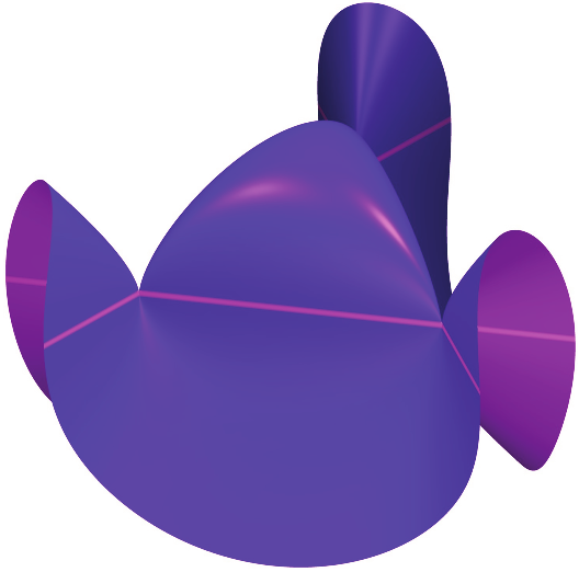
In 2000, Allcock, Toledo, and Carlson showed that $\phi$ extends to an isomorphism between the GIT compactification of $\mathbf{M}$ and the Baily-Borel compactification of $\mathbb{B}_4/\Gamma$, which adds only one point. The associated cubic surface, defined by $\{x_0x_1x_2+x_3^3=0\}$, is depicted in Figure 5. A related isomorphism, involving stable pairs and a toroidal compactification, was recently discovered by L. Schaffler and the authors 7.