Random Numbers: Nothing Left to Chance
Posted March 2008.
The generation of random numbers is too important to be left to chance. --Robert Coveyou
David Austin
Grand Valley State University
david at merganser.math.gvsu.edu
It is often said that mathematics is about understanding patterns and that these patterns are what makes mathematics beautiful. This article, however, is about how mathematics may be used to create, or at least simulate, randomness, the lack of patterns. Surprisingly, we will see that it is difficult to create random behavior (in fact, the words "create randomness" may sound a little jarring) and to determine when we have successfully done it.
We will focus on constructing random sequences of numbers. There are many reasons why we might want to do this. For centuries, people have used randomness--a coin toss, for instance--to make important decisions. Of course, many states run lotteries that use a sequence of random numbers to determine the recipients of huge amounts of money.
Some readers may remember the draft lottery used during the Vietnam war. In 1969, the days of the year were ordered by drawing pieces of paper, each with a day of the year written on it, from a bin. Young men born on those days drawn first were more likely to be drafted. A statistical analysis later found that, because they were placed in the bin later, days toward the end of the year were more likely to be drawn. In other words, the days were not ordered randomly, and a more mathematical solution was proposed for subsequent years' lotteries.
Currently, random numbers are used to form encryption keys when information needs to be passed securely, say, across the Internet. Random sequences of numbers are also important for simulating real-world phenomena. For instance, a bank that operates a network of ATM machines may wish to test its software by simulating the actions of customers accessing their accounts at random times through random machines.
Random numbers are also used by so-called Monte Carlo methods to obtain numerical approximations to problems that may be too difficult to solve exactly. For instance, imagine that we do not know the area of the unit circle. We could place the unit circle inside a square of known area and randomly add points to the square. The percentage of points that lie inside the circle should approximate the ratio of the area of the circle to the area of the square. The figure below shows 2000 points randomly placed inside a square whose sides have length 2.2, 1308 of which lie inside the circle. The approximate area of the circle is then the area of the square, 4.84, times 1308/2000, which is 3.16536 (the exact area is, of course,  ).
).

Where do random numbers come from?
Most of us already have an intuitive notion of what random numbers are, but, as we'll see, this is a difficult question to answer precisely. Simply said, we should not be able to use the numbers that we have seen to predict which number will come next or to restrict the possibilities. For example, you may wish to think of rolling an ideal die. On each roll, each of the numbers--1, 2, 3, 4, 5, 6--is equally likely to appear. If we roll many times, we may expect to see each of the six possibilities roughly one-sixth of the time. In addition, if we count the number of successive pairs, we would expect to see each of the 36 possible pairs appear with roughly equal frequency. It is possible, however, that we roll the die one thousand times and obtain a "1" each time. Regardless, each number is equally likely to show up on the 1001st time. (This seeming paradox lies behind a well known Dilbert cartoon.)
At first glance, it may seem like a simple thing to generate random numbers. In fact, you may think that humans could do this easily by, for instance, just writing sequences of 0's and 1's in a stream of consciousness. By following this link, you will be able to write a sequence of one hundred 0's and 1's that will be analyzed using a few of the tests we'll encounter later in this article. If your sequence passes these tests, it shares several properties with truly random sequences. However, you will most likely find it difficult to write a sequence that passes these tests. Humans have a difficult time creating random sequences by trying to "act randomly."
Truly random sequences of numbers may be generated by natural phenomena. Indeed, the web site HotBits, makes available random sequences generated by recording the times between the decays of radioactive particles. For instance, the time between two decays is recorded and compared to the time between the next two. If the first time is shorter than the second, a "0" is recorded, but if the first time is longer than the second, a "1" is recorded. In this way, a sequence of random bits, which may be concatenated to form random integers, is produced. Another site, Random.org, works in a similar way by recording the amplitude of atmospheric noise.
An interesting question is whether the digits of  form a random sequence. Numerical evidence, based on looking at trillions of digits, suggests that they do, but not enough is known at this time to say definitively.
Random number generators
While some sequences generated by natural phenomena produce truly random numbers, many applications require that we be able to create random numbers efficiently inside a computer. This may sound impossible: computers simply execute a set of instructions whose output is determined by the input. Since we supply the computer with the instructions and the input, the output is determined by our choices. How can such a number be random?
The answer is that it's not. Instead, our goal is to use a procedure that hides our footprints so that the numbers create the illusion of randomness. More precisely, we want the numbers to share many properties that we would expect a truly random sequence to enjoy. Such a procedure is often called a pseudorandom number generator, since the numbers generated are not truly random, though we will follow convention and use the term random number generator. Our discussion is greatly influenced by Donald Knuth's exposition in Volume 2 of The Art of Computer Programming, cited in the references.
John von Neumann proposed using the following method as one of the first random number generators. Suppose we want to create eight-digit numbers. Begin with an eight-digit number X0, which we call the seed, and create the next integer in the sequence by removing the middle eight digits from X02. For instance, if X0 = 35385906, we find that
X02 = 1252162343440836
so that our next number is X1 = 16234344. If we repeat this a few times we find:
| X0 |
16234344 |
| X1 |
55392511 |
| X2 |
33027488 |
| X3 |
81496359 |
| X4 |
65653025 |
| X5 |
31969165 |
| X6 |
02751079 |
| X7 |
56843566 |
| X8 |
19099559 |
| X9 |
79315399 |
Since it is difficult, at first glance, to find a pattern in these numbers, we may think that this is an appropriate way to find random numbers. In other words, we have created the illusion of randomness through a deterministic process. Further study shows, however, that this is not a good random number generator. Each term in the sequence depends only on its immediate predecessor and there are only a finite number of possible terms. This means that the sequence will inevitably repeat. The problem is that the sequence can get caught in relatively short cycles. For instance, if the number 31360000 appears in the sequence at some point, we end up with this number again after another 99 iterations and this cycle continues indefinitely.
The middle square method may give you the idea to ask the computer to perform a sequence of many, unrelated, random operations. In fact, Knuth constructed an algorithm that used 13 "peculiar" steps to produce the next number in a sequence of 10-digit numbers and found that it was a very poor way to generate random numbers.
I created a simple algorithm to generate two-digit numbers using apparently "random" operations.
- Start with a two digit number whose digits are d1d0.
- Form a new digit r = 10 - (d1+d0) mod 10.
- Form the three digit number s=d1rd0.
- Let
 and form a new two digit number e1e0 where ei is the dith digit in t after the decimal. and form a new two digit number e1e0 where ei is the dith digit in t after the decimal.
- If e0 is larger than 5, replace it with 10 - e0.
- Now find the arctangent of (e1 + 1) / (e0 + 1). Our new two-digit number is formed by the first two digits after the decimal point.
|
What may seem surprising is that this algorithm produces the short cycle 91, 96, 46, 1, 64, 73, 72, 91, ...., and most seeds lead us to this cycle. As Knuth writes, "The moral of the story is that random numbers should not be generated with a method chosen at random [emphasis original]."
Linear congruential generators
Surprisingly, a good source of pseudorandom number generators comes from the linear congruential method, introduced by Derrick Lehmer in 1949. Here we choose
| a modulus: |
m |
| a multiplier: |
a |
| an increment: |
c |
| a starting value: |
X0 |
We then form the next terms in the sequence by
Xn+1 = f (Xn) = (aX n + c) mod m.
At first glance, it is hard to believe this will produce the illusion of randomness. Remember that we want each term of the sequence to appear to be independent of its predecessor. Can we really accomplish this using a linear function? It turns out that the art is in choosing appropriate values of a, c, and m.
Of course, there are only a finite number of possible numbers 0, 1, 2, ..., m - 1 and since one term is determined by its immediate predecessor, the sequence will inevitably form a repeating cycle whose period will be no larger than m. If this period is short, the sequence will quickly begin to repeat, undesirable behavior if are trying to mimic a random sequence. However, the following theorem shows us how we may make the period have the maximal length m. To express this theorem, it is convenient to use the shorthand b = a - 1.
The period of the sequence {Xn} is m if and only if
- c is relatively prime to m.
- b is a multiple of every prime that divides m.
- b is a multiple of 4 if m is a multiple of 4.
|
For example, the choices  ,
,  and c = 64 produce a cyclic sequence of numbers whose period is m=8505. We therefore have
Xn+1 = (106Xn + 64) mod 8505.
Shown below are the first few points (x, f (x)) created using this generator. As you can see, they appear to be randomly placed.

Typically, integers are represented in a computer using 32 bits so it is natural to choose a value of m close to 232. With an appropriate choice of a and c, our sequence will then cycle through most of the integers that the computer can represent.
Notice that a = c = 1 satisfies the hypothesis of this theorem. However, this choice produces the sequence
X0, X0 + 1, X0 + 2, X0 + 3, X0 + 4, ...,
which is hardly random. Clearly, we need another condition, in addition to the maximal period condition, if we are going to create random numbers using this method. A second condition, which we will now describe, will be quantified using the potency of the sequence, which we define to be the smallest integer s such that bs = 0 mod m.
To understand this quantity, begin with X0 = 0 (which will eventually be encountered since the sequence has period m), and notice that
| X1 = (aX0 + c) mod m = c |
| X2 = (ac + c) mod m |
| X3 = (a2c + ac + c) mod m |
| Xn = (an-1c + ... + ac + c) mod m |
| Xn = (an - 1)c / b) mod m |
If we expand an - 1 = (b + 1)n - 1, then we obtain

If the potency is 1, then we have Xn = (cn) mod m. This sequence is certainly not random.
If the potency is 2, then Xn+1 - Xn = (c + cbn) mod m. In other words, the difference between successive terms behaves in a predictable way so that the sequence cannot be considered random.
Continuing this thinking shows that we need the potency to be relatively high to achieve the illusion of randomness. Experimenting shows that a potency of at least 5 is necessary to create useful random numbers. However, a linear congruential sequence with a potency of 5 is not guaranteed to be random.
In our example above, we had  and
and  , which produces a linear congruential sequence of maximal period with potency 5 (the first few points are shown on the left below). In constrast, if we take
  and
and  , we obtain a linear congruential sequence with maximal period and potency 2 (the first few points are on the right).


In spite of the fact that linear congruential sequences are simply defined, the numbers produced are good enough for many applications. In fact, random numbers provided by computer programming languages, such as Java, are often created by linear congruential generators. The choice of the seed X0 is often taken as the current time expressed in milliseconds.
Other methods, besides the linear congruential method, have been proposed for creating random sequences. Two other ideas come to mind. First, we might choose a quadratic function rather than a linear one. Robert Coveyou suggested the function:
Xn+1 = Xn (Xn + 1) mod 2e
and showed that it produced sufficiently random numbers.
Also, we could consider using more than the previous term in the sequence to generate the next. An example is the lagged Fibonacci sequence, suggested by Gerard Mitchell and Donald Moore in 1958:
Xn+1 = (Xn-24 + Xn-55) mod m
once the first 55 terms of the sequence are generated using, say, a linear congruential generator. The appearance of 24 and 55 in this expression, chosen after careful study, guarantees that the sequence has a suitably long period.
How do we recognize random numbers?
If we propose a method for creating random numbers, we need some way to measure how good its results are. We will now describe a few tests that are important but still somewhat inadequate. To get started, we will describe one test and how it is implemented. Then we will describe a collection of subsequent tests that may be implemented in a similiar way.
Let's consider a simple case in which the numbers we generate are either 0 or 1. There are 32 = 25 possible sequences of five numbers, and each group of five numbers belongs to one of six categories depending on whether there are 0, 1, 2, 3, 4, or 5 zeroes. The following table shows ni, the number of these 32 possibilities that have i zeroes and pi, the probability that a sequence of five numbers, chosen at random, has i zeroes.
| i |
ni |
pi |
| 0 |
1 |
1/32 |
| 1 |
5 |
5/32 |
| 2 |
10 |
10/32 |
| 3 |
10 |
10/32 |
| 4 |
5 |
5/32 |
| 5 |
1 |
1/32 |
What we will now describe is known as the chi square test. Given our sequence {Xn} of zeroes and ones, break it into r disjoint groups of five consecutive elements, and denote by ri the number of groups having i zeroes. If our sequence were random, we should have  so we can measure how our sequence differs from a random one by computing (ri - rpi)2. Since p2 is much larger than p0, we should expect that r2 is much larger than r0 and that the corresponding error term should be larger. To avoid giving undue weight to any of the six possibilities we divide (ri - rpi)2 by rpi and form the chi square statistic

as a measure of how our sequence compares to a random sequence. Smaller values of V should more closely resemble a random sequence.
For example, suppose we have
r0 = 10, r1 = 46, r2 = 95, r3 = 107, r4 = 60, r5 = 15,
for which we compute V=4.835. To interpret this number, we may compute V for all possible sequences {Xn} of zeroes and ones of length 5r and ask what percentage p of the sequences have a lower value of V. Of course, implementing this would be rather tedious, but there is a general theory, which will not be described here, that comes to our rescue and enables us to compute an approximate percentage p in a relatively simple way. In our example, we find that we obtain a lower value of V in approximately p = 56% of the other sequences.
Knuth suggests that our sequence fails the test when p < 1% or p > 99% and that we view it with suspicion when either p < 10% or p > 90%. The thought is that if p is too high, then it differs too much from a random sequence to be considered random. If p is too low, it too closely matches the statistics of a random sequence and should therefore be rejected since its characteristics are too similar to those of a random sequence.
Knuth also suggests running the test three different times on different sequences produced by the generator we are testing. If any test gives a suspicious result, we should not view the generator as producing sufficiently random results. In the same way, we may wish to repeat the test many times and determine how closely the percentages p match the uniform distribution; that is, we expect p to be between 0% and 10% about 10% of the time, between 10% and 20% about 10% of the time and so forth.
There is a widely accepted collection of such tests, known as the Diehard tests, that may be performed in a similar way. We list here a few of them. To qualify as a useful random number generator, a method needs to pass all of these tests, and passing one test is no guarantee that it will pass another.
- Frequency test: We would like our numbers to be uniformly distributed so that if the numbers come from 0, 1, 2, ..., m - 1, then each number occurs with roughly equal frequency. In this case, we let ri be the number of times i occurs in our sequence and notice that pi = 1/ m.
Of course, the nonrandom sequence 0, 1, 2, ... would pass this test. We may therefore ask in addition that every pair (i, j) occur in successive elements with equal frequency. Here we let ri,j count the number of times the pair (i, j) occurs in the sequence and note that pi,j = 1/ m2. This is called the 2-distribution test and may be extended to the more general k-distribution test.
- Permutation test: Select some small value for t such as t = 3, break the sequence into disjoint groups of t consecutive elements and assume that no two elements in a group are equal. There are t! possible ways in which the elements are ordered, each of which is equally likely.
- Run test: In this test, we count the length of "runs," portions of the sequence in which the terms either increase monotonically or decrease monotonically.
- Gap test: We fix a range of values, such as 0, 1, 2, ... , m/ 2, and count the number of terms in the sequence separating two terms that appear in this range.
- Poker test: We form the elements in the sequence {Xn} into groups of five consecutive elements and count the number of "poker hands" that we have. These are:
| All different: |
abcde |
| One pair: |
aabcd |
| Two pairs: |
aabbc |
| Three of a kind: |
aaabc |
| Full house: |
aaabb |
| Four of a kind: |
aaaab |
| Five of a kind: |
aaaaa |
- Birthday spacings test: This test was introduced by George Marsaglia in 1984. Think of the terms of the sequence Xn as birthdays and the numbers 0, 1, 2, ..., m - 1 as days of the year. We will study the spacing between the birthdays. To do this, first order the terms in the sequence in nondecreasing order
 and find the spacings
  between the birthdays. We let ri be the number of times i occurs as a spacing.
The spectral test
The tests we've examined so far may be applied to any random number generator and work by examining sequences output by the generator. The spectral test is specifically designed for linear congruential generators and works by studying the output of the generator over the entire period. We first construct the set of all points (x, f (x)) where f is the function defining the generator. For example, if m = 8505,  , and c = 64, we have

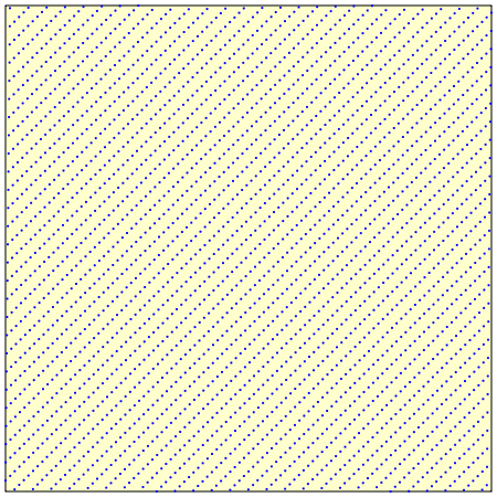
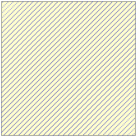
Notice that all the points lie on a finite family of equidistant parallel lines.

In fact, if you look carefully, you will notice that there are many such families of parallel lines containing all the points. This is to be expected since the function f (x) is a linear function. For each family of lines, we may consider the distance between the lines and define d to be the maximum of these distances over all the families of lines. The accuracy of the linear congruential generator is defined to be 1/d.
The accuracy is greater for the generator on the left (which also has a higher potency) since the maximum distance between families of parallel lines is smaller than for the example on the right.
 |
 |
| m = 8505 |
 |
| c = 64 |
|
| m = 8505 |
 |
| c = 64 |
|
To get a feel for why the accuracy should reflect the quality of the random number generator, let's look at the plot of one-twentieth of the points in a period.
Remember that all the points will lie on families of lines. When the accuracy is large, the families of lines are all tightly packed together. When one family of lines is relatively far apart, there is less flexibility for where the points will appear, which makes the sequence appear less random.
The spectral test may be applied in other dimensions as well. For instance, in dimension three, we form the collection of points {(x, f (x), f (f (x))} and notice that these points lie on families of planes. The accuracy is then the reciprocal of the maximum distance between the planes.
There is an efficient algorithm for computing the accuracy in low dimensions. Indeed, the spectral test is the best available for linear congruential generators: all generators that are known to be good pass the spectral test while all generators known to be bad fail it.
Conclusions
As we've seen, it can be hard to generate a sequence of random numbers and hard to determine exactly how random the sequence is. It is also surprising that one of the most popular means for generating random numbers is given by such a simple linear function.
In 1997, Makoto Matsumoto and Takuji Nishimura found a new random number generator, which they named the Mersenne Twister, with the phenomenally large period 219937 - 1. Though it is not safe to use in cryptographical applications, it generates random numbers very efficiently and is now in wide use.
References
- Donald E. Knuth, The Art of Computer Programming, Volume 2, Third Edition, Addison-Wesley, Boston. 1997. Knuth's book is an excellent, comprehensive reference. Start here if you are interested in learning more.
- Stephen Park and Keith Miller, Random Number Generators: Good Ones are Hard to Find, Communications of the ACM, October 1988, Volume 31, Number 10, 1192-1201.
- Makoto Matsumoto and Takuji Nishimura, Mersenne Twister: A 623-dimensionally equidistributed uniform pseudorandom number generator, ACM Transactions on Modeling and Computer Simulation, January 1988, Vol. 8, No. 1, 3-30.
- HotBits, Genuine random numbers, generated by radioactive decay.
- Random.org, a site that provides random numbers obtained through variations in atmospheric noise.
- The Diehard tests, maintained by George Marsaglia at Florida State University.
- Statisticians Charge Draft Lottery Was Not Random, New York Times, January 4, 1970, page 66.
David Austin
Grand Valley State University
david at merganser.math.gvsu.edu
Those who can access JSTOR can find some of the papers mentioned above there. For those with access, the American Mathematical Society's MathSciNet can be used to get additional bibliographic information and reviews of some these materials. Some of the items above can be accessed via the ACM Portal , which also provides bibliographic services.


 ).
).
 form a random sequence. Numerical evidence, based on looking at trillions of digits, suggests that they do, but not enough is known at this time to say definitively.
 and form a new two digit number e1e0 where ei is the dith digit in t after the decimal.
 ,
,  and c = 64 produce a cyclic sequence of numbers whose period is m=8505. We therefore have

 , we obtain a linear congruential sequence with maximal period and potency 2 (the first few points are on the right).
 so we can measure how our sequence differs from a random one by computing (ri - rpi)2. Since p2 is much larger than p0, we should expect that r2 is much larger than r0 and that the corresponding error term should be larger. To avoid giving undue weight to any of the six possibilities we divide (ri - rpi)2 by rpi and form the chi square statistic
 and find the spacings
  between the birthdays. We let ri be the number of times i occurs as a spacing.
