Sales and Chips
Posted September 2005.
If a particular country which manufactured computer chips could find better solutions to large TSP problems, it could manufacture those chips more cheaply...
Joe Malkevitch
York College (CUNY)
malkevitch at york.cuny.edu 
Introduction
What do the problems of designing an efficient drop-off route for individuals who have decided on a group cab ride home from an airport and the manufacture of a computer chip have in common? The answer is that both problems can be formulated in terms of the mathematical problem known as the Traveling Salesman Problem (TSP). (Nowadays, of course, the traveling salesman might well be a traveling saleswoman, but I will use the problem's traditional name.) The phrase "traveling salesman" rightly conjures up the image of a salesman, starting out from his home (or place of business), making his appointed rounds to show off the goods he is selling, and then returning to his starting point. The goal of the salesman and his employer might be different. The salesman, who must travel by car, might want to route himself via his favorite cousin's hometown and perhaps take in an antiques show on the way, while the employer might want to have the salesman follow the cheapest route possible.
It turns out that the traveling salesman problem is not only an important applied problem with many fascinating variants; it also has important ties to theoretical mathematics and computer science.
History and Basic Ideas
As with many historical questions, it is complex to pin down exactly where the TSP as a mathematical problem came from. There is a reference to it as a practical problem in a German book from 1832. Some people credit Karl Menger with popularizing the problem to the European mathematical community in the 1920's. Merrill Flood, who studied at Princeton, also popularized the problem and brought it to the attention of the mathematics and operations research community (in the US). He indicated that he heard of the problem from A. W. Tucker in 1937.
Flood claimed that Tucker had been told about the problem by Hassler Whitney, but when Tucker was asked about this he was unable to confirm or deny it - he no longer remembered!
Whitney also had no recollection of having discussed the problem with Tucker (below).
(Courtesy of Alan Tucker, A. W. Tucker's son)
In any case Flood (whose name is also associated with the theory of games) encouraged the study of the problem by the Rand Corporation. From its earliest days Rand was actively involved in work in operations research and, as we shall see below, there are many operations research problems that take the form of the TSP.
Even before mathematicians looked at this problem there were analytically minded salesmen and their employers who thought about it. Let us look at a very simple example. Suppose the diagram below shows the road distance between the three towns to which Hilda, who sells software to high schools, must travel (starting from home). The numbers near the line segments (edges) in the diagram are the driving distances between the locations.
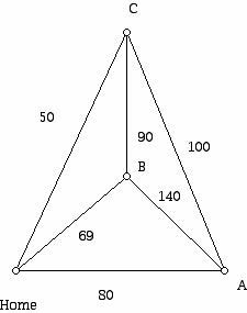
Figure 1 (A 4-city TSP problem)
What we have above is a diagram consisting of dots and lines known as a graph. This is a special kind of graph known as a complete graph because each vertex is joined to every other one. Furthermore, we have assigned to each edge of the complete graph a weight, which could be a time, road distance, cost of a train or airplane ticket, etc. for the trip between the two locations at the endpoints of the edge. Usually these weights are taken as nonnegative numbers (but it is interesting to consider what interpretation might be put on using negative weights) which obey the triangle inequality. This means that given three locations X, Y, and Z the sum of the weights for any pair of the three edges the locations determine is at least as large as the weight on the third edge. (For a distance function, satisfying the triangle inequality is part of the usual definition, as is the requirement that the distance from A to B be the same as the distance from B to A.) In our example, we are assuming that we have a symmetric TSP - the cost in going from X to Y is the same as the cost in going from Y to X - but many interesting applications give rise to an asymmetric TSP in which the cost of going from X to Y may not be the same as the cost in going from Y to X.
The goal in solving a TSP is to find the minimum cost tour, the optimal tour. A tour of the vertices of a graph which visits each vertex (repeating no edge) once and only once is known as a Hamiltonian circuit. Thus, one can think of solving a TSP as finding a minimum cost Hamiltonian circuit in a complete graph with weights on the edges.
It may not even occur to some people that the order in which we visit the various territory towns makes a difference, but one way to see this is to determine all the different tours that one can pick. First, notice one simplification. If one visits the territory towns in the order: Home, A, B, C, Home, then this will be considered the same as the tour where we visit the territory towns in the reverse order: Home, C, B, A, Home. We will consider such pairs of tours the "same," even though there may be pros and cons of various kinds in choosing between the two tours. In terms of total cost, the tours yield the same answer.
In the situation shown in Figure 1, how many TSP tours are there? Since from home one can visit any of three choices, and from there one can visit any of two cities, etc., and using the fundamental principle of counting (which tells us to multiply the number of ways that one can do each component task in the counting problem), we find that there are 3! = 3 x 2 x 1 = 6 routes, which divided by 2 (for the reason described above) gives 3 different routes. For the general complete graph with n vertices, the number of different TSP routes would be:

Returning to the problem in Figure 1 and enumerating the 3 TSP tours we can select the cheapest one:
HABCH which costs 80 + 140 + 90 + 50 = 360
HACBH which costs 80 + 100 + 90 + 69 = 339
HCABH which costs 50 + 100 + 140 + 69 = 359.
Thus, going from Home to A, then to C, then to B and then back Home is best.
So what gives here? Why not enumerate for the general TSP problem involving n cities all the possible routes and select the cheapest? The problem is with the rapid growth of the factorial function (m!) which is involved in the counting of the TSP tours. For even a modest number of cities the best current supercomputers can not enumerate all of the tours! Thus, using brute force to solve even modest-sized TSP problems will not work.
Are there simple algorithms which will yield an optimal solution to the TSP problem? If you were faced with the TSP problem in Figure 1, perhaps you might be tempted to proceed as follows: Go from Home to the closest location and visit next that site not already visited which is cheapest to go to next. This approach is an example of a greedy algorithm. A greedy algorithm makes a "locally" best decision. The question is to see whether or not the locally optimal choices lead to a solution which is globally optimal.
The idea just described is often referred to as the Nearest Neighbor (NN) approach to finding a TSP tour. If we apply NN to the problem in Figure 1 we get the tour HCBAH, not an optimal solution. But, given how fast it is to apply NN for even very large problems we can now ask a new question. Even if NN does not yield an optimal answer to the TSP, does it yield a sufficiently good solution that we can settle for this, given how fast we get a solution? Thus, we are thinking of NN as an approximation algorithm to the TSP problem. There are two well known "measures" that one can use for telling how good an approximation algorithm is. One of these measures refers to how far off the approximation algorithm can be in the worst case. The other measure tries to see how well the approximation algorithm does on an "average case" problem. Sometimes the approximation algorithm approach in mathematics is very gratifying in that one finds very good approximations to what appear to be very hard problems relatively quickly. We will return to this issue below.
Since NN does not always yield an optimal solution to the TSP, let us try another greedy algorithm which might do better. It seems natural that any minimal cost TSP would use cheap edges. So why not try to add the edges in constructing a TSP in order of cheapness? Of course, without being careful about what edges we add we might not get a single circuit which passes through all the vertices. Thus, we need to add the edges in order of increasing cost, subject to the restriction that we never choose more than two edges that meet at a vertex and never form a circuit which does not include all of the vertices. Let us call this greedy algorithm the Sorted Edges Algorithm. If this algorithm is applied to the TSP in Figure 1, we first sort the edges by cost: 50, 69, 80, 90, 100, 140. We can use the edge of weight 50, then the edge of weight 69, but if the edge of weight 80 is added we get three edges at a site, so this is not allowed. Adding the edge of weight 90 would create a circuit of length 3 (not 4) so we can not use that edge. This means that we must complete our tour using the edges of weight 100, and 140. Thus, the tour we obtain is: HCABH. This tour also fails to be optimal.
Algorithms such as Sorted Edges and Nearest Neighbor are fast to implement and easy to understand conceptually but unfortunately are not guaranteed to give optimal solutions. Such fast-to-implement, not-necessarily-optimal algorithms are sometimes referred to as heuristics or heuristic algorithms.
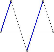
Another approach to taking a current circuit which visits each site once and only once and trying to find a cheaper circuit uses the following ideas. Consider, for example, the circuit below (Figure 2) in a five-vertex complete graph, where the weights of the edges are not shown. What is shown is a circuit which is currently as good a TSP tour as we have been able to find when the weights are taken into consideration. Highlighted in the diagram are two edges which have no vertex in common. These two edges determine 4 vertices (the endpoints of the edges). We can delete the edges shown and join these 4 vertices up with two new edges that transform the circuit shown into another circuit. The two edges used to do this are shown in Figure 3 in blue.
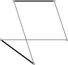
Figure 2
Figure 3
Note that in the diagram above the edges in the circuit in Figure 2 other than the dark black ones are still present. The blue edges are different from the black ones but, when added to the previous edges, yield a circuit. If the two edges which are added have total cost less than the two edges they replace, then the new TSP tour is cheaper than the previous tour. Other heuristics adopt this edge-switching strategy to find improved tours. The example above illustrates what is called the 2-opt approach because switches involving two edges are used. For larger TSP problems one can use a 3-opt strategy where three edges are deleted and 3 new edges added with the goal of lowering the total cost. For modest sized problems the "k-opt" heuristic works quite well.
The Euclidean TSP
An interesting special case of the TSP is to consider the optimal route passing through a collection of n points (sites) in the Euclidean plane (or more generally, n-dimensional Euclidean space). The weights between the points (sites) involved are taken to be the Euclidean distance between the points. If in an optimal tour some pair of edges AC and BD cross as shown below (Figure 4, top), then this can not be an optimal tour. Why? Consider the tour where the edges A'B' and D'C' replace the edges AC and BD in our tour. Let us compare the cost of the tour ACBDA with the tour A'B'C'D'A' (Figure 4, bottom). Note that the edges AC and BD meet at a point Q which is not one of the original sites involved in the TSP. We know that AQ + QB is larger than A'B' (because in the triangle AQB, the sum of any two sides has Euclidean length greater than the third side). Similarly DQ + QC is longer than D'C'. Thus, AQ + QB + DQ + QC is longer than A'B' + D'C'. However AQ + QC = AC and DQ + QB = DB and hence, if we replace AC and DB by A'B' and D'C', we get a shorter tour.

Figure 4
Other special properties of optimal solutions for TSP tours of points in the Euclidean plane depend on the ordering of the points in the convex hull (the points common to all convex sets containing the set) of the set of sites. Thus, the ordering of all sites in an optimal tour must include the vertices of the convex hull in "cyclic order" of the convex hull polygon.
Insights from Computer Science
In attempting to get insights into how hard it is to solve TSP problems, it turns out to be convenient to distinguish between two ways of thinking about the TSP situation. In one perspective, what one has is a decision problem. Given a weighted complete graph with n vertices, locate a tour which visits each vertex once and only once whose total weight is less than a fixed constant k. However, there is also the optimization version of the problem, the one we have emphasized here, where the goal is finding the tour of the vertices once and only once with total weight the smallest possible.
What are researchers to make of the fact that the many attempts to find a simple algorithm to answer these versions of the TSP have failed? One explanation might be that the right clever idea has not yet been found. Another explanation might be that there is no simple or fast algorithm for solving the TSP! During the period that investigations into the TSP as a particular problem in operations research were being pursued, there were tremendous strides being made in computer science. With the advent of low cost commercial computers in the 1950's the problem of designing algorithms to solve complex problems on computers came to the center of the stage. Computers could carry out complex procedures that were not practical to do by hand. Were there principles to be learned in designing good algorithms? What was the fastest algorithm to solve a particular type of problem? These were questions that were part of the emerging new subject of computer science. Within computer science a new discipline sprouted up: complexity theory. Complexity theory deals with trying to classify how hard a problem is to solve on a computer. Among the major issues of concern are how much time and how much space (computer memory) are required to solve a particular problem.
If one tries to solve a TSP (e.g. finding the best tour) which involves 10 cities, it would not be surprising to find that it would require more work than a TSP with 6 cities. On the other hand in comparing two 10-city problems, is it harder to solve a problem whose distances between sites are all in the range from 3,000,000 to 8,000,000 than it is to solve one where the sites are never more than 20 units apart? Since computers at some stage typically change numbers to binary and since numbers which do not exceed 20 can be represented with 5 binary bits while those with 8,000,000 would require many more bits, it is not surprising that there is more "overhead" in working with large numbers than with small numbers. However, does this "overhead" significantly change the amount of work needed to solve a TSP with n cities? Is it the number of cities or the size of the distances between them that contributes in an essential way to the "complexity" of the TSP? In intuitive terms the "size" of many problems can be described with a single number. Other "parameters" associated with the problem are typically not irrelevant but do have a smaller influence on how hard the problem is to solve. How is the amount of work to be measured? For the TSP this parameter n is taken as the number of cities or sites to be visited. All different TSP problems of size n are considered to be equivalently difficult.
To carry out its work, an algorithm has to be given input data in some form. This form is known as a data structure. The data for a graph, for example, might be input into the computer in the form of a matrix or it might be input in the form of lists of vertices to which the vertices of the graph are connected (with a weight attached). For example, for the graph in Figure 5, we could represent the information in either of the two forms below, where not only are we indicating which vertices are connected to which vertices but also the weights on the edges. Thus, the "infinity" symbol in the (A, D) cell means that there is no edge from A to D while the 6 in the the (A, B) cell indicates the edge from A to B has weight 6. For the list representation, if a vertex is not joined to another one, then this vertex is omitted from the list. The idea is to count the number of operations that the algorithm must carry out to obtain its answer. For example, in measuring the complexity of a sorting algorithm where there are nnumbers to sort, one might count how many comparisons and how many interchanges of the numbers in the original list are required to complete the sorting process.
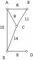
Figure 5

Figure 6 (Matrix representation of Figure 5)
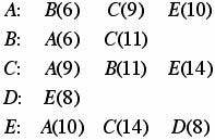
Figure 7 (List representation of Figure 5)
The list representation of a graph with many vertices and few edges will have fewer symbols than the matrix representation for the same graph. Some problems might lend themselves to easier algorithms when the data is given in one data structure rather than another.
While some problems can be solved using very fast algorithms, others turn out to have algorithms whose only known algorithms all take a long time to solve. Some problems have been shown to be so hard that no algorithm to solve them will terminate in a finite amount of time. The situation for the TSP is very interesting. The decision version of the TSP is known to be NP-complete, which means that there is no known polynomial time algorithm for the TSP and that if any of many thousands of problems were found to have a polynomial time algorithm, then there would be a polynomial time algorithm for the TSP. On the other hand, for NP-complete problems there is no proof that an exponential algorithm is required, and a proof for any of these problems that showed exponential work was needed to solve the problem would imply a proof for all of them. Thus, the NP-complete problems are a group of "equally" hard or easy (as measured by polynomial time) problems; we just do not know which.
It is widely believed that no polynomial time algorithm for the TSP will be found. The optimization version of the TSP is known to be NP-hard. This means that the problem is known to be in NP, and if some polynomial time solution to this problem existed, then some (hence, every) NP-complete problem would be solvable in polynomial time. To be in NP means that all problems in NP reduce to this problem in polynomial time. To be in NP means that one can verify (not necessarily find) that a solution given to one is correct in polynomial time. If someone gives a good "guess" for a solution we can very quickly verify that it works.
It is known that the decision TSP problem is NP-complete but there remains the issue of whether one can quickly find a good approximation to the TSP. There are two different senses in which one might mean a good approximation. On the one hand, if one applies an algorithm one might be interested in knowing that on the average one gets a good solution. On the other hand one might be interested in knowing in the worst case that one can not be too far off. Thus, if one could show that one could apply an algorithm for the TSP for n cities, and that no matter what the distances involved are, one can find in polynomial time a solution which is no more than 1.01 x OPT, where OPT denotes the best weight solution that exists, one would be much happier than if that method did no better than find a solution which is no more than 1.5 x OPT.
A relatively recent breakthrough shows that a polynomial time approximation scheme exists for a special type of TSP, namely when the weights (costs) in the problem are Euclidean distances, whereas for general values no such approximation scheme exists.
The important thing to keep in mind here is that the optimization version of the TSP is so important that solutions must be found to TSP problems which are either provably optimal even though it takes a long time to find them, or which are provably relatively good approximations. For example, if a particular country which manufactured computer chips could find better solutions to large TSP problems, it could manufacture those chips more cheaply, which would make its product more competitive in comparison with a country which could not solve the TSP as efficiently.
Variations on a Theme
Mathematicians are trained to take an important problem and find related problems that are also of interest. The variations that mathematicians find for a problem are carried out on many fronts. This reflects the fact that the methods that have proved useful in solving a particular problem are often useful in carrying out related or "nearby" problems. One way to extend what one knows is in the applied arena: Take the problem of interest and change to an application related to the original one. For example, one might have originally wanted to solve a problem for a salesman but realize that the problem of picking up children and taking them to a day camp is a related problem but one with the constraint that one can not exceed the size of the minibus. As another example, we have considered applications where a tour is found which starts and ends at the same site and visits each vertex once and only once. What about the problem of starting at a site, visiting each vertex once and only once, but ending at a different site?
One also can vary the problem in a mathematical framework independent of whether there is a natural application of this variant. For example, as we posed the original problem it can be stated:
Find a minimum cost tour for a (simple circuit) of sites making up a weighted complete graph.
The features of this problem are that:
(a). One is seeking a circuit,
(b). The objective function is to minimize the sum of the weights of the edges in the circuit, and
(c). The weights are assumed to be "abstract distances." (Thus, they are symmetrical and obey the triangle inequality.)
Above, we changed Condition (a) for applications reasons. We could also change Condition (a) even if we could think of no application. Surprisingly, these new problems often do find applications in the future, and they may suggest new theoretical issues as well.
We get many interesting variants by changing Condition (b). For example, the Bottleneck Traveling Salesman Problem (bottleneck TSP) arises as a variant of the usual TSP by changing the objective function. It is stated as follows: Find the Hamiltonian circuit in a weighted graph with the minimal length of the longest edge. Now one can try to answer questions such as the computational complexity of this variant (e.g. Is the bottleneck TSP NP-complete?) and to find heuristics for the problem. Since this problem was generated on theoretical grounds, one might also try to see if there are applications for this problem as well. It might seem natural that one would want to use as the objective function having a tour which minimizes the shortest edge, but what about a tour which maximizes the shortest edge? Not only have researchers investigated this question, but it turns out to have an application to how to position rivets in airplane wings!
Finally, we might consider changing the nature of the weights or distances involved. We briefly did this above when considering the special version of the TSP where the distances were Euclidean distances. It is known that this problem is also NP-complete. Of course, we can also vary several of the conditions above at once. For example, suppose we want to find a TSP tour where the total length of the tour is as large as possible for points described by ordered pairs of real numbers. It turns out that in two dimensions if the length of the tour involves distances which obey the "taxicab" metric, then the problem can be solved in polynomial time, unlike the situation where the distance between the pairs is given by Euclidean distance and one wants to minimize the length of the tour.
The TSP is also a sub-problem of many large operations research problems. For example, a school district may use a fleet of minibuses to pick students up from specified street corners and deliver them to and from school. If the bus has a capacity of C, one may want to take the locations where the various students can be picked up and divide them into groups where each group contains at most C students congregating at those locations. Now one wants to arrange a TSP for each one of those minibuses. The goal in all of this is to design a system which minimizes the total cost in getting the students to school, or perhaps some other optimization function, such as minimizing the average time the students spend in a bus. Problems of this type embed the TSP in a broader collection of problems called vehicle routing problems. Typically vehicle routing problems incorporate more "specialized" features than merely the cost of getting between pick up and delivery points. They deal with the capacity of the vehicle carrying the goods or passengers (e.g. an airport van can seat at most 6 people or a small truck can carry at most a ton of products). They might also have to take into account "alternate side of the street parking" regulations, such as those used in many large cities, which would affect the pattern for employing trucks to make deliveries to stores.
These are only some of the many examples of how mathematics is being used to find increasingly efficient solutions to harder and more subtle operations research problems, thereby improving all of our lives.
References
Applegate, D. and R. Bixby, V. Chvatal, W. Cook, TSP cuts which do not conform to the template paradigm, In Computational Combinatorial Optimization, Optimal or Provably Near-Optimal Solutions, LNCS, Volume 2241, Springer-Verlag, 2001, p. 261-304.
Arkin, E. and M. Bender, J. Mitchell, S. Skiena, The lazy bureaucrat scheduling problem, Proceedings of the 6th International Workshop on Algorithms and Data Structures, 1999, p. 122.-133.
Arkin, E., and Y-J. Chiang, J. Mitchell, S. Skiena, T-C. Yang, On the maximum scatter traveling salesperson problem, SIAM J. Computing, 29 (1999) 515-544.
Arora, S., Polynomial time approximation schemes for Euclidean traveling salesman and other geometric problems, Journal of ACM, 45 (1998) 753-782.
S. Arora, and M. Grigni, D. Karger, P. Klein, A. Woloszyn, A polynomial-time approximation scheme for weighted planar graph TSP, Proc. 9th Annual ACM-SIAM Symposium on Discrete Algorithms, 1998, p. 33-41.
Arora, S. and C. Lund, R. Motwani, M. Sudan, M. Szegedy, Proof verification and hardness of approximation problems, Journal of the ACM, 45 (1998) 501-555.
Ausiello, G. and E. Feuerstein, S. Leonardi, L. Stougie, M. Talamo, Algorithms for the on-line traveling salesman, Algorithmica, 29 (2001) 560-581.
Baltz, A. and A. Srivastav, Approximation algorithms for the Euclidean bipartite TSP, Operations Research Letters, 33 (2005) 403-410.
Barvinok, D. Johnson, G. Woeginger, R. Woodroofe, The maximum traveling salesman problem under polyhedral norms, Proceedings of the 6th IPCO Conference on Integer Programming and Combinatorial Optimization, 1998, p. 195-201.
Barvinok, A. E. Gimadi, A. Serdyukov, The maximum traveling salesman problem, in The Traveling Salesman Problem and its Variations, G. Gutin and A. Punnan, (eds.), Kluwer, Dordrecht, 2002, p. 585-607.
Bianco, L. and A. Mingozzi, S. Ricciardelli, Dynamic programming strategies and reduction techniques for the traveling salesman problem with time windows and precedence constraints, Operations Research, 45 (1997) 365-377.
Charikar, M. and B. Raghavachari, The finite capacity dial-A-ride problem, In Proceedings of the 39th Annual IEEE Symposium on the Foundations of Computer Science, 1998.
Chiang, Y-J, New approximation results for the maximum scatter TSP, Algorithmica, 41 (2005) 309-341.
Christofides, N., Worst-case analysis of a new heuristic for the traveling salesman problem, Report 388, Graduate School of Industrial Administration, Carnegie Mellon U, 1976.
Clarke, G. and J. Wright, Scheduling vehicles from a central depot to a number of delivery points, Operations Research 12 (1964) 568-581.
Dantzig, G. and J. Ramser, The truck dispatching problem, Management Science 6 (1959) 80-91.
Deineko, V. and G. Woeginger, The convex-hull-and-k-line traveling salesman problem: a solvable case, Information Processing Letters, 59 (1996) 295-301.
Deineko, V. and M. Hoffmann, Y. Okamoto, G. Woeginger, The traveling salesman problem with few inner points, Proceedings of the 10th International Computing and Combinatorics Conferences, LNCS Volume 3106, Springer-Verlag, 2004, 268-277.
Deineko, V. and R. van Dal, G. Rote, The convex-hull-and-line traveling salesman problem: a solvable case, Info. Proc. Lett., 59 (1996) 295-301.
Fekete, S. Simplicity and harness of the maximum traveling salesman problem under geometric distances, Proceedings of the 10th ACM-SIAM Symposium on Discrete Algorithms, 199, p. 337-345.
Flood, M., The traveling-salesman problem, Oper. Res. 4 (1956) 61-75.
Gamarnik, D. and M. Lewenstein, M. Sviridenko, An improved upper bound for the TSP in cubic 3-edge connected graphs, Operations Research Letters, 33 (2005) 467-474.
Garfinkel, R, Minimizing wallpaper waste, Part I: a class of traveling salesman problems, Oper. Res. 25 (1977) 741-751.
Garfinkel, R. and K. Gilbert, The bottleneck traveling salesman problem: algorithms and probabilistic analysis, J. Assoc. Comput. Mach., 25 (1978) 435-438.
Garey, M. and D. Johnson, Computers and Intractability, W. H. Freeman, New York, 1979.
Grigni, M. and E. Koutsoupias, C. Papadimitriou, An approximation scheme for planar graph TSP, In, Proc. IEEE Symposium on the Foundations of Computer Science, 1995, 640-645.
Gutin, G. and A. Punnen, (eds.), The Traveling Salesman Problem and Its Variations, Kluwer, Nowell, MA., 2002.
D. Johnson and L. McGeoch, The Traveling Salesman Problem: A Case Study in Local Optimization, in Local Search in Combinatorial Optimization, E. H. L. Aarts and J.K. Lenstra (ed), Wiley, 1997, p. 215-310.
Karuno, Y. and H. Nagamochi, T. Ibaraki, A 1.5-approximation for single-vehicle scheduling problem on a line with release and handling times, In Japan-U.S.A. Symposium on Flexible Automation, July, 1998, p. 1363-1366.
Kruskal, J., On the Shortest Spanning Subtree of a Graph and the Traveling Salesman Problem, Proc. Amer. Math. Soc. 7 (1956) 48-50.
Lawler, E., A solvable case of the traveling salesman problem, Math. Programming 1 (1971) 267-267.
Lawler, E. and J. Lenstra, A. Rinnooy Kan, D. Shmoys, (eds.) The Traveling Salesman Problem: A Guided Tour of Combinatorial Optimization, Wiley, New York, 1985.
Lewenstein, M. and M. Sviridenko, A 5/8-approximation algorithm for the maximum asymmetric TSP, SIAM J. Discrete Math., 17 (2003) 237-248.
Lin, S. "Computer Solutions of the Traveling Salesman Problem." Bell System Tech. J. 44 (1965) 2245-2269.
Martello, S. and P. Toth, Knapsack Problems: Algorithms and Computer Implementations, Wiley, Chichester, 1990.
Miller, C. and A. Tucker, R. Zemlin, Integer programming formulations and traveling salesman problems, J. of the ACM, 7 (1960) 326-329.
Papadimitrious, C., The Euclidean TSP is NP-complete, Theoretical Comput. Sci., 4 (1977) 237-244.
Papadimitriou, C., The complexity of the Lin-Kernighan heuristic for the traveling salesman problem, SIAM J. on Computing, 21 (1992) 450-465.
Papadimitriou, C. and S. Vempala, On the approximability of the traveling salesman problem (extended abstract). Proceedings of STOC 2000, p. 126-133.
Platzman, L. K. and Bartholdi, J. J. "Spacefilling Curves and the Planar Traveling Salesman Problem." J. Assoc. Comput. Mach. 46, 719-737, 1989.
Reinelt, G. "TSPLIB--A Traveling Salesman Problem Library." ORSA J. Comput. 3, 376-384, 1991.
Rosenkrantz, D. J.; Stearns, R. E.; and Lewis, P. M. "An Analysis of Several Heuristics for the Traveling Salesman Problem." SIAM J. Comput. 6, 563-581, 1977.
Shmoys, D. and D. Williamson, Analyzing the Held-Karp TSP bound: A monotonicity property with application, IPL 35 (1990) 281-285.
Toth, P. and D. Vigo, (eds.), The Vehicle Routing Problem, SIAM, Philadelphia, 2002.
Trevisan, L., When Hamming meets Euclid: the approximability of geometric TSP and Steiner tree, SIAM J. Computing, 30 (2000) 475-485.
Tsitsiklis, J., Special cases of the traveling salesman and repairman problems with time windows, Networks, 22 (1992) 263-282.
Woeginger, G., Exact algorithms for NP-hard problems: a survey, in Combinatorial Optimization - Eureka! You shrink!, Lecture Notes in Computer Science, Vol. 2570, 2003, p. 185-207.
Joe Malkevitch
York College (CUNY)
malkevitch at york.cuny.edu
NOTE: Those who can access JSTOR can find some of the papers mentioned above there. For those with access, the American Mathematical Society's MathSciNet can be used to get additional bibliographic information and reviews of some these materials. Some of the items above can be accessed via the ACM Portal, which also provides bibliographic services.