How to Grow and Prune a Classification Tree
In what follows, we will describe the work of Breiman and his colleagues as set out in their seminal book "Classification and Regression Trees." Theirs is a very rich story, and we will concentrate on only the essential ideas...
Introduction
It's easy to collect data these days; making sense of it is more work. This article explains a construction in machine learning and data mining called a classification tree. Let's consider an example.
In the late 1970's, researchers at the University of California, San Diego Medical Center performed a study in which they monitored 215 patients following a heart attack. For each patient, 19 variables, such as age and blood pressure, were recorded. Patients were then grouped into two classes, depending on whether or not they survived more than 30 days following the heart attack.
Assuming the patients studied were representative of the more general population of heart attack patients, the researchers aimed to distill all this data into a simple test to identify new patients at risk of dying within 30 days of a heart attack.
By applying the algorithm described here, Breiman, Freidman, Olshen, and Stone, created a test consisting of only three questions---what is the patient's minimum systolic blood pressure within 24 hours of being admitted to the hospital, what is the patient's age, does the patient exhibit sinus tachycardia---to identify patients at risk. In spite of its simplicity, this test proved to be more accurate than any other known test. In addition, the importance of these three questions indicate that, among all 19 variables, these three factors play an important role in determining a patient's chance of surviving.
Besides medicine, these ideas are applicable to a wide range of problems, such as identifying which loan applicants are likely to default and which voters are likely to vote for a particular political party.
In what follows, we will describe the work of Breiman and his colleagues as set out in their seminal book Classification and Regression Trees. Theirs is a very rich story, and we will concentrate on only the essential ideas.
Classification trees
Before we start developing a general theory, let's consider an example using a much studied data set consisting of the physical dimensions and species of 150 irises. Here are the data for three irises out of the 150 in the full data set:
|
Sepal Length |
Sepal Width |
Petal Length |
Petal Width |
Species |
|
5.1 |
3.5 |
1.4 |
0.2 |
Iris-setosa |
|
4.9 |
3.0 |
1.4 |
0.2 |
Iris-setosa |
|
5.6 |
3.0 |
4.5 |
1.5 |
Iris-versicolor |
Together, the four measurements form a measurement vector, ${\bf x} = (x_1, x_2, x_3, x_4)$ where
-
$x_1$, sepal length in cm,
-
$x_2$, sepal width in cm,
-
$x_3$, petal length in cm, and
-
$x_4$, petal width in cm.
Our full data set contains three species of irises---Iris Setosa, Iris Versicolor, and Iris Virginica---equally represented among the 150 irises in the set. The species will be denoted by $Y$. Here is the table above for the three irises selected from the data set of 150, but now using the variables:
|
$x_1$ |
$x_2$ |
$x_3$ |
$x_4$ |
$Y$ |
|
5.1 |
3.5 |
1.4 |
0.2 |
Iris-setosa |
|
4.9 |
3.0 |
1.4 |
0.2 |
Iris-setosa |
|
5.6 |
3.0 |
4.5 |
1.5 |
Iris-versicolor |
From this data set, which we call the learning sample, we will construct a classifier, a function $Y=d({\bf x})$ that predicts an iris' species from its measurement vector. Ideally, the classifier should accurately predict the species of irises we have yet to meet.
Though there are many ways in which a classifier could be constructed, we will build a binary tree known as a decision tree from the learning sample.

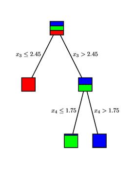
Given a measurement vector ${\bf x}$, we begin at the root of the tree. Each non-terminal node asks a question of the measurement vector. For instance, the root of the tree asks if $x_3\leq 2.45$. If the answer is "yes," we move to the left child of the node; if "no," we move to the right. Continuing in this way, we eventually arrive at a terminal node and assign the species $Y=d({\bf x})$ as indicated.
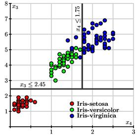
Notice that the tree only uses the two variables $x_3$ and $x_4$ and ignores $x_1$ and $x_2$. Shown below is a plot of the $(x_3,x_4)$ values of the 150 irises in the learning sample along with the root of the decision tree.
We see that the first question $x_3 \leq 2.45$ completely separates the Iris-setosa samples from the others.
Then the question $x_4\leq 1.75$ looks like the best possible split of the remaining samples.
Notice that our classifier is not perfect; however, asking only two questions misclassifies only 4% of the irises in the learning sample. If we are optimistic, we may hope for similar success with new data. Also, the decision tree reveals the role that the petal length and petal width play in the classification.
Comments?
Growing the decision tree
Now that we know where we're headed, let's see how to construct the decision tree from the learning sample. The learning sample contains a set of $N$ cases, each composed of a measurement vector and the class to which the case belongs. Using $j$ to denote one of the classes, we write the learning sample as ${\cal L} = \{({\bf x}_k, j_k)\}_{k=1}^N$.
In the construction process, we will work with a node $t$ and a set of associated cases ${\cal L}(t)$. For instance, we begin the construction with $t_1$, the root of the tree, to which all cases in the learning sample are assigned: ${\cal L}(t_1) = {\cal L}$.
If all the cases in ${\cal L}(t)$ belong to the same class $j$, then there is no more work to do with this node. We declare $t$ to be a leaf of our tree; should a measurement vector $\bf x$ fall through the decision tree to this node, we declare that $d({\bf x}) = j$.
However, if there are cases in ${\cal L}(t)$ belonging to more than one class, we will consider using a question of the form "Is ${\bf x}_i \leq c$?" to split the cases in ${\cal L}(t)$ into two sets. Cases for whom the answer is "yes" form ${\cal L}(t_L)$, associated to the left child of $t$; those for whom the answer is "no" form ${\cal L}(t_R)$, asociated to the right child.

We must consider whether there is any benefit to splitting the node $t$, and if there is, how can we choose the best possible split. To assess the quality of a split, we introduce $i(t)$, which measures the "impurity" of the cases in ${\cal L}(t)$. If all the cases in ${\cal L}(t)$ belong to a single class, $t$ is a "pure" node so that $i(t) = 0$. Conversely, the maximum impurity should occur when there is an equal number of each class in ${\cal L}(t)$. When splitting a node, we seek to decrease the impurity as much as possible.
To define $i(t)$, we introduce $p(j|t)$, the probability that a case in ${\cal L}(t)$ belongs to class $j$. Notice that $\sum_j p(j|t) = 1$.
A typical measure of the impurity is the Gini measure: $$i(t) = i_G(t) = 1-\sum_j p(j|t)^2.$$
This clearly satisfies $i(t) = 0$ when all the cases belong to a single class and it has a maximum when $p(j|t)$ are all equal, meaning that each class is equally represented in ${\cal L}(t)$.
To measure a split's change in impurity, we use the probabilities $p_L$ and $p_R$ that a case in $t$ falls into $t_L$ or $t_R$ and compute: $$\Delta i = i(t) - p_Li(t_L) - p_Ri(t_R).$$
It is straightforward to see that $\Delta i \geq 0$, which means that a split will never increase the total impurity.
Recall that the splits we consider have the form $x_i \leq c$. Furthermore, notice that two values, $c_1, c_2,$ $c_1 < c_2,$ define the same split if there are no cases in ${\cal L}(t)$ with $c_1< ({\bf x}_k)_i \leq c_2$. This means that we only need to consider splits that have the form $x_i \leq ({\bf x}_k)_i$ where ${\bf x}_k$ is the measurement vector of a case in ${\cal L}(t)$.
Therefore, the number of splits we must consider equals the number of cases in ${\cal L}(t)$ times the number of variables. Though this is potentially a large number, this process is computationally feasible in typical data sets. We therefore consider every possible split and declare the best split to be the one that maximizes $\Delta i$, the decrease in impurity.
Comments?
Misclassification costs
Beginning with the root, the tree will grow as we continue to split nodes. Since we wish to stop the splitting process when we have the best possible tree, we need some way to assess the quality of a decision tree.
Suppose we are constructing our decision tree and arrive at a node $t$. We may declare this node to be a leaf and assign all the cases in ${\cal L}(t)$ to a single class $j(t)$. Often, we choose $j(t)$ so that the smallest number of cases are misclassified, in which case $j(t)$ is the class having the largest number of cases in ${\cal L}(t)$.
Sometimes, however, some misclassifications are worse than others. For instance, in the study of heart attack patients described in the introduction, it is better to err on the side of caution by misclassifying a patient as at risk of dying within 30 days rather than misclassifying a patient that is truly at risk.
For this reason, we frequently introduce a misclassification cost $C_{ji}$ that describes the relative cost of misclassifying a class $i$ case as class $j$. For instance, Breiman and his colleagues empirically arrived at a ratio of 8 to 3 between the cost of misclassifying an at-risk patient as a survivor to the cost of misclassifying a survivor as at risk.
Notice that $C_{jj} = 0$ since there is no cost in classifying a class $j$ case as class $j$.
With this in mind, choose $j(t)$ to be the class that minimizes the misclassification cost of all the cases in ${\cal L}(t)$; that is, $j(t)$ minimizes: $$ M(j) = \sum_{i} C_{ji}p(i|t). $$
The misclassification cost at node $t$ is defined to be this minimum: $$ r(t) = \sum_{i}C_{j(t)i}p(i|t). $$
When all costs are equal, $r(t) = 1-\max_{j} p(j|t)$, which represents the probability that a class in ${\cal L}(t)$ is not in the largest class and is therefore misclassified.
To assess the quality of a decision tree $T$, we will consider the total misclassification cost of $T$. If $t$ is a leaf of $T$, the contribution that $t$ makes to the total misclassification cost is $$ R(t) = r(t)p(t), $$ where $p(t)$ is the probability that a class falls through the tree to $t$.
Denoting the leaves of $T$ by $\tilde{T}$, we then write $$ R(T) = \sum_{t\in\tilde{T}} R(t) = \sum_{t\in\tilde{T}} r(t)p(t). $$
Given any splitting of a node, it is straightforward to check that the misclassification cost only decreases after a split: $$ R(t) \geq R(t_L) + R(t_R). $$ This is intuitively clear since the chance that the class of a given case lies in the majority can only increase when the node is split.
Two thoughts may come to mind now:
-
Why not use the misclassification cost, rather than the impurity, to determine the best way to split a node? That is, why not split node $t$ so as to minimize the misclassification cost?
Some simple examples show that choosing splits that minimize $R(T)$ does not necessarily lead to the best long-term growth of the tree. For instance, Breiman and his colleagues demonstrate the following two splits:

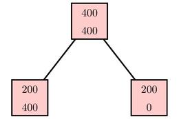
Both splits misclassify 25% of the cases: $R(T) = 0.25$. However, the split shown on the right seems better since it leads to a pure node containing only one class. This node has $R(t) = 0$ as it classifies its cases perfectly; such a split often leads to better decision trees in the long run. We therefore use the impurity, as described above, to determine the best split.
-
Why not split so long as we can lower the impurity? Clearly, one option is to continue splitting until every node is pure. For instance, using the 150 irises as a learning sample, we obtain the following tree:

Doing so, however, gives some cases in the learning sample undue weight in the decision tree and weakens the predictive power of any trend our tree has detected. This is known as overfitting. For instance, let's consider the plot of our data again

paying special attention to the boxed region in the center:
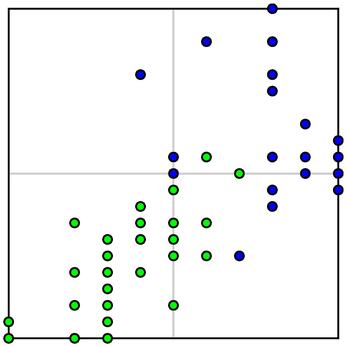
Generally speaking, it appears that Iris-versicolor samples have smaller values of $x_3$ and $x_4$ when compared to Iris-virginica. Since there is some overlap in the two species, however, it seems better to accept that our tree will necessarily misclassify some cases in the overlap.
To determine when we stop splitting, we could require that a split produces a decrease in the impurity greater than some threshold. Empirical evidence, however, shows that it is possible to have one split that produces a small decrease in impurity while subsequent splits have larger decreases. A threshold-stopping criterion would therefore miss the later desirable splits.
Due to these considerations, Brieman and colleagues instead continue splitting until $i(T) = 0$, meaning every leaf is a pure node. This also implies that the misclassification cost $R(T) = 0$.
This tree, which we denote $T_{max}$, probably overfits the data; we therefore "prune" $T_{max}$ to obtain a better tree by minimizing the cost-complexity, as we will next describe.
Comments?
The cost-complexity measure
As we have seen, the tree $T_{max}$ likely overfits the data giving undue weight to some cases in the learning sample. Notice that $T_{max}$ has a small misclassification cost $R(T)$ and a large number of leaves. We would like to find another tree with a smaller number of leaves at the expense of allowing $R(T)$ to rise somewhat. That is, we seek a balance between the number of leaves and the misclassification cost.
The complexity of a tree $T$ is the number of its leaves $|\tilde{T}|$ and the cost-complexity measure is $$ R_\alpha(T) = R(T) + \alpha |\tilde{T}|, $$
where $\alpha \geq 0$ is the complexity parameter. Of course, when $\alpha = 0$, $R_0(T) = R(T)$, the misclassification cost. As we increase $\alpha$, however, we begin to impose an increasing penalty on trees having a large number of leaves. Trees that minimize $R_\alpha$ will therefore have a low misclassification cost and a small number of leaves.
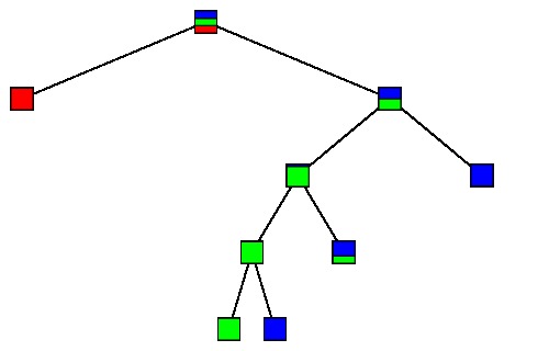
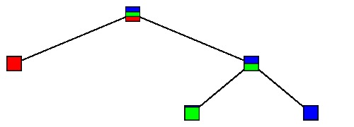
We seek trees that minimize $R_\alpha$ by pruning $T_{max}$. In other words, we choose a node $t$ and eliminate its children and their children and so on; in the new tree, $t$ is a leaf. For example, this tree

is obtained by pruning the tree below.
If $T'$ is obtained from $T$ by pruning, we will write $T'\preceq T$.
For a fixed value of $\alpha$, we say that $T'$ is an optimally pruned tree of $T_{max}$ if $$ R_\alpha(T') = \min_{T\preceq T_{max}} R_\alpha(T). $$
Moreover, we define $T(\alpha)$ to be the smallest optimally pruned tree of $T_{max}$; that is, if $ R(T(\alpha))=R(T')$, then $T(\alpha) \preceq T'$. It is relatively straightforward, using some of the ideas we are about to describe, to see that there is a smallest optimally pruned tree $T(\alpha)$ and that it is unique.
Recall that $R(t) \geq R(t_L) + R(t_R)$, which means that splitting a node decreases the misclassification cost while increasing the number of leaves. Increasing the complexity parameter $\alpha$ imposes a greater penalty on the number of leaves. This is reflected in the following fact, which is straightforward to verify:
If $\alpha_1 \leq \alpha_2$, then $T(\alpha_1) \succeq T(\alpha_2)$.
That is, as we increase $\alpha$, we obtain a sequence of trees $T_i$ such that $$ T_{max} \succeq T_1 \succ T_2 \succ \ldots \succ T_m = \{t_1\}. $$
In fact, it is fairly easy to generate this sequence of trees. For instance, let's begin with $T_1$, which is obtained from $T_{max}$ by pruning all leaves that do not increase the misclassification rate.
If $t$ is a node of $T_1$, consider $R_\alpha(t) = R(t) + \alpha$; that is, if we prune $T_1$ to obtain $T'$ by declaring $t$ to be a leaf, then $R_\alpha(t)$ is the contribution to $R_\alpha(T')$ from the leaf $t$.
Also, consider the tree $T_t$ consisting of $t$ and all its descendants in $T_1$. Removing $T_t$ from $T_1$ leaves the same set of nodes as removing $t$ from $T'$. That means that $$ R_\alpha(T_1) - R_\alpha(T_t) = R_\alpha(T') - R_\alpha(t) $$ or $$ R_\alpha(T_1) - R_\alpha(T') = R_\alpha(T_t) - R_\alpha(t). $$
Since we seek trees that minimize $R_\alpha$, consider the case when $R_\alpha(T')\leq R_\alpha(T_1)$, which is equivalent to $R_\alpha(t)\leq R_\alpha(T_t)$. This makes sense intuitively: in this case, we can lower $R_\alpha$ by replacing $T_t$ with the single node $t$.
Then we have \[ \begin{eqnarray*} R_\alpha(t) & \leq & R_\alpha(T_t) \\ R(t) + \alpha & \leq & R(T_t) + \alpha\left|\tilde{T_t}\right| \\ \frac{R(t) - R(T_t)}{\left|\tilde{T_t}\right| - 1} &\leq &\alpha \end{eqnarray*} \]
Therefore, we consider the function on the nodes of $T_1$ $$g_1(t) = \frac{R(t) - R(T_t)}{\left|\tilde{T_t}\right| - 1},$$ and define $$ \alpha_1 = \min_{t\in T_1-\tilde{T_1}} g_1(t). $$
If $\alpha < \alpha_1$, we cannot lower $R_\alpha$ by pruning $T_1$, which shows that $T(\alpha) = T_1$. The tree $T_2=T(\alpha_1)$ is obtained by pruning $T_1$ at all the nodes $t$ for which $g_1(t) = \alpha_1$.
The next tree $T_3$ is obtained by pruning $T_2$ in the same manner.
Looking at the learning sample of 150 irises, we find the following trees:
|
$\large T_1$ |
 |
|
$\large T_2$ |
 |
|
$\large T_3$ |
 |
|
$\large T_4$ |
 |
|
$\large T_5$ |
 |
|
$\large T_6$ |
 |
Comments?
Choosing the right-sized tree
To summarize, we used our learning sample to grow a large tree $T_{max}$, which was then pruned back to obtain a sequence of trees $$T_1 \succ T_2 \succ \ldots T_m=\{t_1\}.$$
The trees in this subsequence are our candidates for our decision tree. How do we choose which is the best?
One answer is obtained by using a test sample, a set of cases that is independent of the learning sample. For each tree $T_i$, we run all the cases in the test sample through the decision tree and find the misclassification cost $R^{ts}(T_i)$ on the test sample. The optimal decision tree is the one that minimizes $R^{ts}(T_i)$.
In practice, we usually begin with a large sample that is randomly split into a learning sample and a test sample. In this case, Breiman and his colleagues describe a preferable alternative known as $V$-fold cross-validation.
Once again, ${\cal L}$ is our original data set. We randomly divide ${\cal L}$ into $V$ disjoint subsets ${\cal L}_v$, $v=1, 2,\ldots, V$ of roughly equal size. In practice, Breiman and his colleagues recommend choosing $V$ to be approximately 10.
For each $v$, let $\overline{{\cal L}^v}$ be the complement of ${\cal L}^v$ in ${\cal L}$. For each $v$ and complexity parameter $\alpha$, we use $\overline{{\cal L}^v}$ to construct the tree $T^v(\alpha)$. In the case that $V=10$, $T^v(\alpha)$ is constructed using approximately 90% of the data. It is therefore reasonable to assume that its predictive accuracy will be close to that of $T(\alpha)$ constructed using the entire data set ${\cal L}$.
Since the cases in ${\cal L}^v$ are not used in the construction of $T^v(\alpha)$, we may use ${\cal L}^v$ as an independent test sample and define $N_{ij}^v(\alpha)$ to be the number of class $j$ cases in ${\cal L}^v$ classified as class $i$ by $T^v(\alpha)$.
Then $N_{ij}(\alpha) = \sum_v N_{ij}^v(\alpha)$ is the number of class $j$ cases in ${\cal L}$ classified as $i$ from which we evaluate the cross-validated misclassification cost. This we expect to closely reflect the misclassification cost of $T(\alpha)$ constructed from the full data set ${\cal L}$.
As before, we find the value of $\alpha$ that minimizes the cross-validated misclassification cost and choose $T(\alpha)$ for our decision tree.
Comments?
Summary
Besides laying out the construction of the decision tree as described here, Breiman and his colleagues provided a theoretical statistical foundation justifying its use. In addition, they implemented this construction in the software now known as CART and successfully applied it to situations such as the study of heart attack patients.
This technique is much more general and robust than is described here. For instance, it is possible to incorporate splits given by more general linear functions of the variables. Variables are allowed to be categorical rather than numerical, and CART deals well with cases having some missing variables. Also, the use of "regression trees" allows the predictions to be numerical rather than categorical as well.
In spite of the fact that CART was introduced some thirty years ago, its use, especially with some more recent enhancements, is still widespread today.
References
-
Leo Breiman, Jerome Friedman, Richard Olshen, and Charles Stone. Classification and Regression Trees. Wadsworth International Group. 1984
-
Xindong Wu et al. Top 10 algorithms in data mining. Knowledge and Information Systems, vol. 14, pp. 1-37, 2008.
-
UCI Machine Learning Repository, a collection of frequently used test data sets.
-
Salford Systems' implementation of CART.
-
An Interview with Leo Breiman, in which he describes some of the problems that led to the development of CART and some of his colorful life.
 David Austin