How to Differentiate with a Computer
Automatic differentiation has been used for at least 40 years and then rediscovered and applied in various forms since. It seems, however, to not be as well known as perhaps it should be. ...
Introduction
Though it can seem surprising and even mysterious, we're all aware that mathematical ideas, which spring from our human imagination, can help us solve problems we see in the world around us. What is recognized less frequently is that it can be challenging putting a mathematical idea to work effectively.
Newton's method provides a familiar example.
|
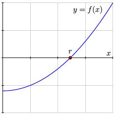
Suppose we have a function $f(x)$ and we would like to find the point $r$ where $f(r) = 0$ as shown in the figure.
|
 |
|
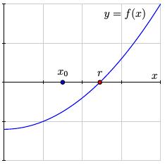
We make an initial guess $x_0$ as to the location of $r$.
|
 |
|
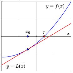
We then construct the linearization $y=L(x)$ to the function $y=f(x)$ at the point corresponding to $x_0$. Solving the equation $f(x) = 0$ may be difficult, but solving the linear equation $L(x) = 0$ is simple.
|
 |
|
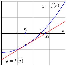
It's not hard to see that the solution to the equation $L(x) = 0$ is $$ x_1 = x_0 - \frac{f(x_0)}{f'(x_0)}. $$ We then repeat this process by linearizing at $x_1$ and solving again to find $$ x_2 = x_1 - \frac{f(x_1)}{f'(x_1)}. $$
|
 |
If we have made a reasonable initial guess $x_0$ and continue in this way, we create a sequence $\{x_n\}$, where $$ x_{n+1} = x_n - \frac{f(x_n)}{f'(x_n)}, $$ that converges to the root $r$; that is, $x_n\to r$. In this way, we can find the root $r$ to any degree of accuracy that we wish.
Suppose now that we would like to automate this process by creating a program that efficiently implements Newton's method for a function $f$ supplied by a user. Our program needs to compute values for both the function $f$ and its derivative $f'$ at the points $x_n$.
We have some options for computing the derivative $f'$. First, we could ask a computer algebra system, such as Mathematica, Matlab, or Sage, to compute the derivative $f'$ symbolically and then evaluate $f'$ at the points $x_n$. There are, however, a couple of disadvantages to this approach. First, finding the derivative symbolically, and then evaluating the resulting expression, can be computationally expensive. This is especially true if we have an application requiring a higher derivative. Second, we need to be able to write a symbolic expression for the function. If the function values appear as the result of a computational algorithm, it may be difficult or even impossible to express $f$ symbolically.
A second approach is to estimate the derivative numerically using, say, a central difference $$ f'(x_j) \approx \frac{f(x_j+h)-f(x_j-h)}{2h} $$ for a small value of $h$. Of course, this approach only produces an approximation to the derivative, and this particular approximation is plagued by numerical instability. For instance, if $f(x)=e^x$ and we approximate $f'(0)=1$ using the central difference, we find:
| $h$ |
$\displaystyle\frac{f(h)-f(-h)}{2h}$ |
| 1e-12 |
1.00000008274 |
| 1e-13 |
1.00003338943 |
| 1e-14 |
0.999755833675 |
| 1e-15 |
0.999200722163 |
| 1e-16 |
1.05471187339 |
What we would prefer is a technique that evaluates the derivative at a point in the same amount of time and with the same accuracy with which we evaluate the function at a point. The subject of this column, known as automatic or algorithmic differentiation, provides just such a technique.
Automatic differentiation has been used for at least 40 years and then rediscovered and applied in various forms since. It seems, however, to not be as well known as perhaps it should be. We will begin by describing how dual numbers lead to a simple implementation of an automatic differentiation technique.
Dual numbers and the forward mode of differentiation
To automate the computation of derivatives, we define the dual numbers as the set of numbers $a+b\epsilon$ where $a$ and $b$ are real numbers along with the requirement that $\epsilon^2 = 0$. These numbers seem naturally related to differentiation if we think, as the notation suggests, of $\epsilon$ as an extremely small, but positive, quantity whose square is so small that it can be safely ignored. This formalism allows us to consider small linear changes while ignoring quadratic and higher-order side effects.
For comparison, the complex numbers are the set of numbers $a+bi$ where $a$ and $b$ are real and $i^2 = -1$. Just as the ring of complex numbers can be represented by the ring of $2\times2$ matrices having the form $ \left[\begin{array}{cc} a & -b \\ b & a \\ \end{array}\right], $ we can represent the ring of dual numbers using $2\times2$ matrices of the form $ \left[\begin{array}{cc} a & 0 \\ b & a \\ \end{array}\right] $.
Basic arithmetic operations are straightforward: $$ \begin{aligned} (a+b\epsilon) + (c+d\epsilon) & {}={} (a+c) + (b+d)\epsilon \\ (a+b\epsilon) (c+d\epsilon) & {}={} ac + (ad+bc)\epsilon \\ \frac{a+b\epsilon}{c+d\epsilon} & {}={} \frac ac + \frac{bc - ad}{c^2}\epsilon. \\ \end{aligned} $$ Notice that a dual number $c+d\epsilon$ only has a multiplicative inverse if $c\neq 0$.
We now find that $$ (a+b\epsilon)^2 = a^2 + 2ab\epsilon. $$ That is, if we consider the squaring function $f(x) = x^2$, then $f(a+b\epsilon) = f(a) + f'(a)b\epsilon$. The binomial theorem says that a similar result is true for any power function: $$ (a+b\epsilon)^n = a^n + na^{n-1}b\epsilon. $$
This suggests that we extend the definition of a real function $f(x)$ to dual numbers $a+b\epsilon$, where $f$ is differentiable at $a$, as $$ f(a + b\epsilon) = f(a) + f'(a)b\epsilon. $$
Many familiar properties of derivatives are compatible with this definition.
-
Product rule: If $f(x) = g(x)h(x)$, then $$ \begin{aligned} f(a+b\epsilon) & {}={} g(a+b\epsilon) h(a+b\epsilon) \\ & {}={} \left(g(a) + g'(a)b\epsilon\right)\left(h(a)+ h'(a)b\epsilon\right) \\ & {}={} g(a)h(a) + \left(g'(a)h(a) + g(a)h'(a)\right)b\epsilon, \\ \end{aligned} $$ which gives us the product rule: $f'(a) = g'(a)h(a) + g(a)h'(a)$.
-
Chain rule: Similarly, if we have a composite function $f(x) = g(h(x))$, then $$ \begin{aligned} f(a+b\epsilon) & {}={} g\left(h(a+b\epsilon)\right) \\ & {}={} g\left(h(a)+h'(a)b\epsilon\right) \\ & {}={} g(h(a)) + g'(h(a))h'(a)b\epsilon, \\ \end{aligned} $$ which leads to the chain rule: $f'(a) = g'(h(a))h'(a)$.
|
Now we can put this to use. Suppose that we would like to find the derivative of the function $f(x) = x\sin(x^2)$ at the point $a=3$. The evaluation of this function can be represented by the graph shown on the right. Notice that we have introduced auxilliary variables to decompose the function into simpler parts.
|
 |
We will find $f'(3)$ by evaluating $f(3+\epsilon) = f(3) + f'(3)\epsilon$; that is, we set $x=3+\epsilon$ to obtain $$ \begin{aligned} u & {}={} x^2 \\ & {}={} (3+\epsilon)^2 = 3^2 + 2\cdot 3\epsilon \\ & {}={} 9 + 6\epsilon. \end{aligned} $$ Then $$ \begin{aligned} v & {}={} \sin(u) \\ & {}={} \sin(9+6\epsilon) \\ & {}={} \sin(9) + 6\cos(9)\epsilon, \end{aligned} $$ and finally $$ \begin{aligned} w & {}={} x\sin(v) \\ & {}={} (3+\epsilon)(\sin(9)+6\cos(9)\epsilon) \\ & {}={} 3\sin(9) + (\sin(9) + 18\cos(9))\epsilon. \end{aligned} $$ Therefore, we have evaluated both $f(3) = 3\sin(9)$ and $f'(3) = \sin(9) + 18\cos(9)$ with a single computation.
Suppose we are finding the solutions of an equation $f(x)=0$ using Newton's method; we therefore need to evaluate both $f(a)$ and $f'(a)$ at a collection of points. Using dual numbers, we find both quantities with roughly twice as much work as needed to evaluate $f(a)$ alone. If we had used symbolic differentiation instead, we would have invested the effort to find $f'(x) = \sin(x^2) + 2x^2\cos(x^2)$ and then still needed to evaluate $f'(3)$. Dual numbers provide the same result with the same accuracy while bypassing the symbolic computation of $f'(x)$.
Even better, it is easy to implement this technique in many object-oriented programming languages using operator overloading. We first define a data type that models dual numbers and then extend the definition of simple operators such as +, *, sin, exp, log and so forth to accept dual numbers. Since any function can be written by combining these operators, it is then possible to write simple code, such as
    x = 3 + Epsilon
    print x * sin(x**2)
Because this process proceeds through the function graph in the same order as which we evaluate the function, we call this the forward mode of automatic differentation. We will later meet the reverse mode.
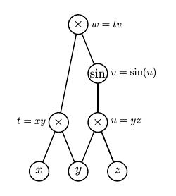 Another simple extension allows us to compute gradients of multivariable functions. Consider, for instance, the function $f(x,y,z) = xy\sin(yz)$ whose gradient we wish to evaluate at $(x,y,z) = (3,-1,2)$. We set $$ \begin{aligned} x & {}={} 3 + \epsilon[1,0,0] \\ y & {}={} -1 + \epsilon[0,1,0] \\ z & {}={} 2 + \epsilon[0,0,1]. \\ \end{aligned} $$
This leads to $$ \begin{aligned} t {}={} & \left(3+\epsilon[1,0,0]\right)\left(-1+\epsilon[0,1,0]\right) = -3 + \epsilon[-1,3,0] \\ \\ u {}={} & \left(-1+\epsilon[0,1,0]\right)\left(2+\epsilon[0,0,1]\right) = -2 + \epsilon[0,2,-1] \\ \\ v {}={} & \sin\left(-2+\epsilon[0,2,-1]\right) = \sin(-2)+\epsilon \cos(-2)[0,2,-1] \\ \\ w {}={} & \left(-3+\epsilon[-1,3,0]\right) \left(\sin(-2)+\epsilon \cos(-2)[0,2,-1]\right) \\ {}={} & -3\sin(-2) + \\ & \epsilon[-\sin(-2), 3\sin(-2)-6\cos(-2), 3\cos(-2)]. \\ \end{aligned} $$
We therefore see that $$ \begin{aligned} f(3,-1,2) & {}={} -3\sin(-2) \\ \nabla f(3,-1,2) & {}={} [-\sin(-2), 3\sin(-2)-6\cos(-2), 3\cos(-2)]. \\ \end{aligned} $$
As before, this is also easily implemented in many of your favorite programming languages through operator overloading. If $f$ is a function of $n$ variables, the amount of computation required here is about $n+1$ times the amount required to simply evaluate the function.
Comments?
Higher derivatives
What if we would like to find higher derivatives of a function $f(x)$? We can extend these ideas by thinking in terms of Taylor polynomials. Rather than working with dual numbers $a+b\epsilon$ where $\epsilon^2 = 0$, we can work with polynomials $$a_0 + a_1\epsilon + \ldots + a_N\epsilon^N$$ and define $\epsilon^{N+1} = 0$. This will allow us to compute the derivatives of a function $f(x)$ through its $N^{th}$ derivative $f^{(N)}$.
We define $$f(a+\epsilon) = f_0 + f_1\epsilon + f_2\epsilon^2 + \ldots + f_N\epsilon^N, $$ where $f_j = \frac{f^{(j)}(a)}{j!}$. Dealing with arithmetic operations is straightfoward. For instance, if $f(x) = g(x)h(x)$, then $$ \begin{aligned} f(a+\epsilon) & {}={} g(a+\epsilon)h(a+\epsilon) \\ & {}={} (g_0 + g_1\epsilon + \ldots + g_N\epsilon^N) (h_0 + h_1\epsilon + \ldots + h_N\epsilon^N) \\ & {}={} f_0 + f_1\epsilon + \ldots + f_N\epsilon^N. \end{aligned} $$ As expected, we see that $$ f_k = \sum_{j=0}^k g_jh_{k-j}, $$ which, when expressed in terms of derivatives, yields the product rule for higher derivatives.
Quotients are a little more work. Suppose that $f(x) = g(x)/h(x)$ so that we have $$f(a+\epsilon) = \frac{g(a+\epsilon)}{h(a+\epsilon)} = \frac{g_0 + g_1\epsilon + \ldots + g_N\epsilon^N} {h_0 + h_1\epsilon + \ldots + h_N\epsilon^N}. $$ The trick here is to write $g(x) = f(x)h(x)$ so that we have $$ \begin{aligned} g_0 + g_1\epsilon + \ldots + g_N\epsilon^N {}={} & \left(f_0 + f_1\epsilon + \ldots + f_N\epsilon^N\right) \\ & \left(h_0 + h_1\epsilon + \ldots + h_N\epsilon^N\right). \end{aligned} $$ By multiplying these series, we find $$ \begin{aligned} g_0 & {}={} f_0h_0, & f_0 & {}={} \frac{g_0}{h_0} \\ g_1 & {}={} f_0h_1+f_1h_0, & f_1 & {}={} \frac{1}{h_0}\left(g_1-f_0h_1\right) \\ \end{aligned} $$ and so on.
Composition with elementary functions also requires some thought. For instance, suppose we have $f(x) = e^{g(x)}$. The idea is to write the function as a solution to a differential equation: $$f'(x) = e^{g(x)}g'(x) = f(x)g'(x).$$ Evaluating at $a+\epsilon$, we have $$ \begin{aligned} f_1 + 2f_2\epsilon+\ldots+Nf_N\epsilon^{N-1} {}={} & \left(f_0 + f_1\epsilon + \ldots + f_N\epsilon^N\right) \\ & \left(g_1 + 2g_2\epsilon + \ldots + Ng_N\epsilon^{N-1}\right). \end{aligned} $$ We know that $f_0 = e^{g_0}$. We then find that $$ \begin{aligned} f_1 & {}={} f_0 g_0 \\ 2f_2 & {}={} 2f_0g_2 + f_1g_1 \\ \end{aligned} $$ and so on. Notice that we only need to evaluate the exponential once to find $f_0$ and that the other coefficients are found using only multiplications and additions.
Now if we have the function $f(x) = e^{-x^2}$ and would like to find the $10^{th}$ derivative $f^{(10)}(2)$, we have $$ \begin{aligned} f(2+\epsilon) & {}={} e^{-(2+\epsilon)^2} \\ & {}={} e^{-4-4\epsilon - \epsilon^2} \\ & {}={} 0.01832 - 0.07326\epsilon + \ldots -0.00233\epsilon^9+ 0.00101\epsilon^{10}, \\ \end{aligned} $$ which tells us that $$ \begin{aligned} f^{(9)}(2) = (-0.00233)9! = -845.16, \\ f^{(10)}(2) = (0.00101)10! = 3670.75. \\ \end{aligned} $$ Though we have only written the derivatives with a few significant digits, the algorithm computes these derivatives exactly.
Remember that we only need to learn how to compose series with a limited number of functions. It turns out that all the functions we need arise as the solutions of differential equations. For instance, if $f(x) = \arctan(g(x))$, then $f'(x) = \frac{1}{1+g(x)^2}g'(x)$ and we can find the coefficients $f_j$ by multiplying the series for $1/(1+g(x)^2)$ and $g'(x)$.
The reverse mode of automatic differentiation
Earlier, we demonstrated how to find the gradient of a multivariable function using the forward mode of automatic differentiation. If there are $n$ variables, then the amount of computation is roughly $n+1$ times the amount of work required to evaluate the function itself. The reverse mode of automatic differentiation provides a more efficient way to find the partial derivatives.
|
Let's look at our earlier example of the function $f(x,y,z) = xy\sin(yz)$ and find the partial derivatives at the point $(3,-1,2)$.
|
|
|
We first make a pass through the graph in the forward direction to evaluate the auxilliary variables.
|
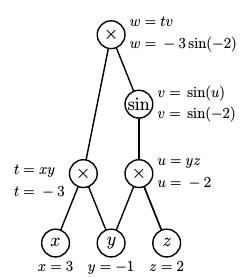 |
We now introduce what are called adjoint variables to record the partial derivatives of the top node with respect to the other nodes. For instance, $$ \begin{aligned} \bar{x} & {}={} \frac{\partial w}{\partial x} \\ \bar{u} & {}={} \frac{\partial w}{\partial u} \\ \end{aligned} $$ We now work our way down the graph beginning with $\bar{w} = \frac{\partial w}{\partial w} = 1$. Then $$ \begin{aligned} \bar{v} & {}={} \frac{\partial w}{\partial v} = t = -3 \\ \bar{t} & {}={} \frac{\partial w}{\partial t} = v = \sin(-2) \\ \bar{u} & {}={} \frac{\partial w}{\partial v}\frac{\partial v}{\partial u} = \bar{v}\cos(u)=-3\cos(-2) \\ \bar{x} & {}={} \frac{\partial w}{\partial t}\frac{\partial t}{\partial x} = \bar{t}y = -\sin(-2) \\ \end{aligned} $$ so we find that $\frac{\partial w}{\partial x} = -\sin(-2)$. In the same way, $$ \begin{aligned} \bar{y} & {}={} \frac{\partial w}{\partial t}\frac{\partial t}{\partial y} + \frac{\partial w}{\partial u}\frac{\partial u}{\partial y} \\ & {}={} \bar{t}x + \bar{u}z \\ & {}={} 3\sin(-2) -6\cos(-2) \\ \end{aligned} $$ and lastly $$ \bar{z} = \frac{\partial w}{\partial u}\frac{\partial u}{\partial z} = \bar{u}y = 3\cos(-2). $$
Though there are several ways to implement the reverse mode, we will just describe one here. We can form a system of linear equations, one for each adjoint variable, as we move through the function graph. Assuming that we are finding the partial derivatives at $(x,y,z)=(3,-1,2)$, we have $$ \begin{aligned} \bar{x} & {}={} -\bar{t} \\ \bar{y} & {}={} 3\bar{t} + 2\bar{u}\\ \bar{z} & {}={} -\bar{u} \\ \bar{t} & {}={} v\bar{w} \\ \bar{u} & {}={} \cos(u)\bar{v} \\ \bar{v} & {}={} 3\bar{w} \\ \bar{w} & {}={} 1. \\ \end{aligned} $$ If we form the vector ${\mathbf x} = \left[\begin{array}{ccccccc} \bar{x} & \bar{y} & \bar{z} & \bar{t} & \bar{u} & \bar{v} & \bar{w} \\ \end{array}\right]^T$ formed from the adjoint variables and the matrix $$ A = \left[\begin{array}{ccccccc} 1 & 0 & 0 & 1 & 0 & 0 & 0 \\ 0 & 1 & 0 & -3 & -2 & 0 & 0 \\ 0 & 0 & 1 & 0 & 1 & 0 & 0 \\ 0 & 0 & 0 & 1 & 0 & 0 & -v \\ 0 & 0 & 0 & 0 & 1 & \cos(u) & 0 \\ 0 & 0 & 0 & 0 & 0 & 1 & -3 \\ 0 & 0 & 0 & 0 & 0 & 0 & 1 \end{array}\right], $$ then we have $A{\mathbf x} = \left[\begin{array}{ccccccc} 0 & 0 & 0 & 0 & 0 & 0 & 1 \\ \end{array}\right]^T. $ Since $A$ is an upper triangular matrix, this can easily be solved by back substitution. In fact, $A$ is typically a sparse matrix, which means that the equation can be easily solved for ${\mathbf x}$.
With some work, it's possible to show that the effort required to perform the computations in the reverse mode is always less than four times the effort required to evaluate the function. When the function has many variables, this represents a considerable savings over the forward mode.
Comments?
Summary
This has been a very brief introduction to the theory of automatic differentiation. In particular, we have not touched on many of the issues related to the implementation of these ideas in a computing environment. This is quite an active area of investigation, which may be explored in the references given below.
We have also not described the many and varied applications of automatic differentiation, though it shouldn't be surprising that a technique for computing derivatives efficiently and with accuracy would be exceptionally useful. Uses include optimization, gradient descent, and sensitivity analysis. Indeed, Nick Trefethen includes automatic differentiation in his list of 29 great numerical algorithms.
Mathematicians justifiably describe their discipline as providing theoretical tools for solving important real-world problems. The gap between the theory and its uses, however, is not always slight. This article hopes to illuminate an example of what is required to bridge this gap.
References
-
Andreas Griewank and Andrea Walther. Evaluating Derivatives: Principles and Techniques of Algorithmic Differentiation, Second Edition, SIAM, Philadelphia. 2008.
-
Richard D. Neidinger. Introduction to Automatic Differentiation and MATLAB Object-Oriented Programming. SIAM Review, Vol. 52, No. 3, 545-563. 2010.
This overview of the subject includes ideas for introducing automatic differentiation into an undergraduate numerical analysis class.
-
Louis B. Rall. Perspectives on Automatic Differentiation: Past, Present, and Future? in Automatic Differentiation: Applications, Theory, and Implementations, Bücker et al (editors), 1-14. Springer, Berlin. 2006.
-
Shaun Forth, Paul Hovland, Eric Phipps, Jean Utke, and Andrea Walther (editors) Recent Advances in Algorithmic Differentiation. Springer, Berlin, 2012.
-
Andreas Griewank. Who Invented the Reverse Mode of Differentiation? Documenta Math, Extra Volume ISMP, 389-400. 2012.
-
Nick Trefethen. Who invented the greatest numerical algorithms? 2005.
-
Community Portal for Automatic Differentiation.
A wide variety of resources for those interested in learning more about automatic differentiation, its uses, and its implementations.
Comments?
 David Austin