From Pascal's Triangle to the Bell-shaped Curve
Posted May 2010.
In this column we will explore this interpretation of the binomial coefficients, and how they are related to the normal distribution represented by the ubiquitous "bell-shaped curve."...
Tony Phillips
Stony Brook University
tony at math.sunysb.edu
Pascal's Triangle
Blaise Pascal (1623-1662) did not invent his triangle. It was at least 500 years old when he wrote it down, in 1654 or just after, in his Traité du triangle arithmétique. Its entries C(n, k) appear in the expansion of (a + b)n when like powers are grouped together giving C(n, 0)an + C(n, 1)an-1b + C(n, 2)an-2b2 + ... + C(n, n)bn; hence binomial coefficients. The triangle now bears his name mainly because he was the first to systematically investigate its properties. For example, I believe that he discovered the formula for calculating C(n, k) directly from n and k, without working recursively through the table. Pascal also pioneered the use of the binomial coefficients in the analysis of games of chance, giving the start to modern probability theory. In this column we will explore this interpretation of the coefficients, and how they are related to the normal distribution represented by the ubiquitous "bell-shaped curve."
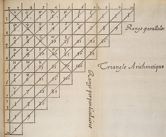
Pascal's triangle from his Traité. In his format the entries in the first column are ones, and each other entry is the sum of the one directly above it, and the one directly on its left. In our notation, the binomial coefficients C(6, k) appear along the diagonal Vζ. Image from Wikipedia Commons.
Factorial representation of binomial coefficients
The entries in Pascal's triangle can be calculated recursively using the relation described in the caption above; in our notation this reads
C(n+1, k+1) = C(n, k) + C(n, k+1).
But they can also be calculated directly using the formula C(n, k) = n! / [k! (n-k)!]. The modern proof of this formula uses induction and the fact that that both sides satisfy the same recursion relation. The factorial notation n! was only introduced at the beginning of the 19th century; Pascal proceeds otherwise. He first establishes his "twelfth consequence:" In every arithmetical triangle, of two contiguous cells in the same base [diagonal] the upper is to the lower as the number of cells from the upper to the top of the base is to the number of cells from the lower to the bottom of the base, inclusive [in our notation, C(n, k) / C(n, k-1) = (n-k+1) / k ]. He proves the twelfth consequence directly from the recursive definition (in the first recorded explicit use of mathematical induction!), and then uses it iteratively to establish
C(n, k) = C(n, k-1) (n-k+1) / k
C(n, k-1) = C(n, k-2) (n-k+2) / (k-1)
...
C(n, 1) = C(n, 0) n / 1 = n;
and so finally
C(n, k) = n(n-1) ...(n-k+1)/ k(k-1) ... 1, a formula equivalent to our factorial representation.
The shape of the rows in Pascal's triangle
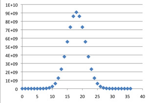
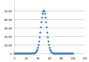
The numbers in Pascal's triangle grow exponentially fast as we move down the middle of the table: element C(2k, k) in an even-numbered row is approximately 22k / (πk)1/2. The following graphs, generated by Excel, give C(n, k) plotted against k for n = 4, 16, 36, 64 and 100. They show both the growth of the central elements and a general pattern to the distribution of values, which suggests that a linear rescaling could make the middle portions of the graphs converge to a limit.
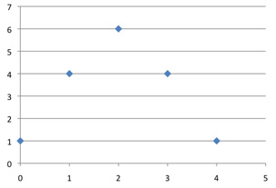
C(4, k)
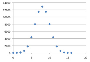
C(16, k)
C(36, k)
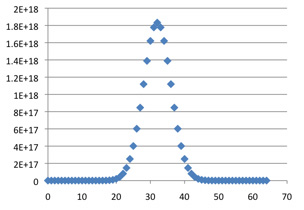
C(64, k)
C(100, k)
As k varies, the maximum value of C(n, k) occurs at n / 2. For the graphs of C(n, k) to be compared as n goes to infinity their centers must be lined up; otherwise they would drift off to infinity. Our first step in uniformizing the rows is to shift the graph of C(n, k) leftward by n / 2; the centers will now all be at 0.
The estimate mentioned above for the central elements (it comes from Stirling's formula) suggests that for uniformity the vertical dimension in the plot of C(n, k) should be scaled down by 2n / n1/2. Now 2n = (1+1)n = C(n, 0) + C(n, 1) + ... + C(n, n), which approximates the area under the graph; to keep the areas constant (and equal to 1) in the limit we stretch the graphs horizontally by a factor of n1/2.
With these translations and rescalings, the convergence of the central portions of the graphs becomes graphically evident:
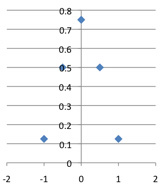
C(4, k)*2 / 2^4, plotted against (k-2) / 2
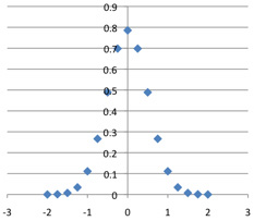
C(16, k)*4 / 2^16, plotted against (k-8) / 4.
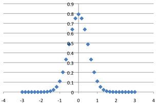
C(36, k)*6 / 2^36, plotted against (k-18) / 6.
C(64, k)*8 / 2^64, plotted against (k-32) / 8.

C(100, k)*10 / 2^100, plotted against (k-50) / 10.
Probabilistic interpretation
Our experiment is an example of the Central Limit Theorem, a fundamental principle of probability theory (which brings us back to Pascal). The theorem is stated in terms of random variables. In this case, the basic random variable X has values 0 or 1, each with probability 1/2 (this could be the outcome of flipping a coin). So half the time, at random, X = 0, and the rest of the time X = 1. The mean or expected value of X is E(X) = μ = 1/2 (0) + 1/2 (1) = 1/2 . Its variance is defined by σ2 = E(X2)-[E(X)]2 = 1/4, so its standard deviation is σ = 1/2. The n-th row in Pascal's triangle corresponds to the sum X1 + ... + Xn, of n random variables, each identical to X. The possible values of the sum are 0, 1, ..., n and the value k is attained with probability C(n, k)/2n. [So, for example, if we toss a coin four times, and count 1 for each head, 0 for each tail, then the probabilities of the sums 0, 1, 2, 3, 4 are 1/16, 1/4, 3/8, 1/4, 1/16 respectively.] This set of values and probabilities is called the binomial distribution with p = (1-p) = 1/2. Its has mean μn = n/2 and standard deviation σn = n1/2/2. In our normalizations we have shifted the means to 0 and stretched or compressed the axis to achieve uniform standard deviation 1/2. The Central Limit Theorem is more general, but it states in this case that the limit of these normalized probability distributions, as n goes to infinity, will be the normal distribution with mean zero and standard deviation 1/2. This distribution is represented by the function
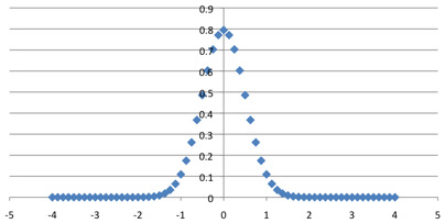
f(x) = 2/(2π)1/2 e-2x2
(its graph is a "bell-shaped curve") in the sense that the probability of the limit random variable lying in the interval [a,b] is equal to the integral of f over that interval.

The normal distribution with μ = 0 and σ = 1/2.
Suppose you want to know the probability of between 4995 and 5005 heads in 10,000 coin tosses. The calculation with binomial coefficients would be tedious; but it amounts to calculating the area under the graph of C(10000, k) between k = 4995 and k = 5005, relative to the total area. This is equivalent to computing the relative area under the normalized curve between (4995-5000) / 100 = -.05 and (5005-5000) / 100 = .05; to a very good approximation this is the integral of the normal distribution function f(x) between -.05 and .05, i.e. 0.0797.
[Correction, May 2017: Three instances of 4005 were changed to 4995. Thanks to a careful reader for the correction--Tony.]
[Correction, December 2018: The value of the last integral has been corrected. Thanks to Art Benis--Tony]
Tony Phillips
Stony Brook University
tony at math.sunysb.edu

